平行公理和微分幾何平行移動(Parallel Transport)
by allenlu2007
垂直和平行都是幾何最重要的基石。
- 垂直的局部性質很直接,兩直線相交,夾角為 90 為垂直。一般人隨手可以畫出垂直相交線,即使在曲面也不例外。垂直的微分定義是兩直線切向量內積為 0.
- 平行的概念看似直接,兩直線永不相交。在歐幾里德平面幾何很容易想像。兩個問題:(A) 這樣平行直線唯一嗎?或一定存在嗎? (B)平行是否有局部的微分定義?
- (A) 的回應就是平行公理;(B)的回應就是平行移動 (parallel transport).
歐幾里得平面幾何五大公理。最後一個公理就是平行公理:一條直線線外一點只能做出唯一平行直線。
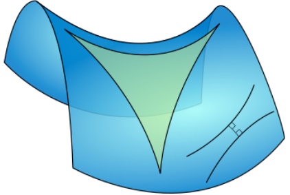
俄國數學家羅巴切夫斯基 (Lobachevsky) 一輩子想要其他公理證明平行公理或者用更直觀的公理取代平行公理都未能成功。後來用反證法:一條直線外一點一定會有兩條或兩條以上的平行直線,試圖找出矛盾。但卻發現邏輯自洽。因而開創非歐幾何學。我們現在知道這其實對應雙曲面幾何如下。這是一個馬鞍面,立起來就是一個雙曲面。雙曲面上的"直線“線外一點可以找到無數 diverged “直線”,和原來的“直線”永不相交,因此可以有無數條平行線。
黎曼則另闢蹊徑開拓黎曼幾何學。對應(橢圓)球面幾何。球面上所有的“直線”都是 中心在球心的封閉大圓。因此所有的“直線”都相交。平行公理變成一條直線外一點沒有任何平行直線。常見的誤區是球面的緯線是平行線。緯線除了赤道是“直線”,其他的緯線都是球面上的“曲線”,不能視為平行直線!
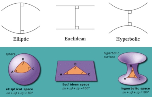
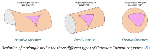
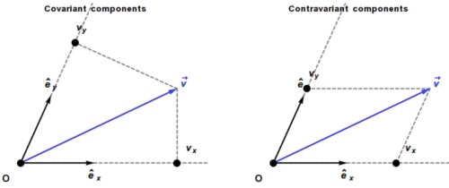
下圖很好的總結三種幾何學。
曲面幾何和曲率
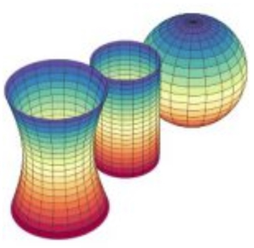
曲面幾何可以定義曲率。曲率乍看之下是把一個曲面放在更高維空間(外)顯出的性質。
例如上圖是把二維的曲面放在(嵌入)三維的歐氏空間,可以明顯看出不同的曲面。同時可以定量的描述這個曲面的曲率。例如球面的曲率非常直觀和球的半徑相反。越小的球,曲率越大。但球面曲率是一個整體的性質,還是每一點(和其鄰近點)的性質?曲率是和半徑成反比,還是和半徑平方成反比?
先回顧二維歐氏平面上的一維曲線。很明顯曲線上每一點(和其鄰近點)都可以定義“線曲率” 

再回到二維曲面,曲面上每一點都有無限條曲面上的曲線相交於這一點。每一條曲線都有本身的“線曲率”,可以是正或負。高斯曲率定義二維曲面每一點的“曲面曲率” 


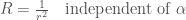
以完美球面為例,每一點所有相交曲線的線曲率都一樣。都是大圓(圓心即是球心)半徑的倒數。所以球面每一點的高斯曲率 
如果是非完美球面,例如橢圓球面半徑為 

再考慮雙曲面幾何。每一點相交曲線的”線曲率“必定有正有負,
外顯和內稟曲率
So far so good!
檢查高斯曲率在平面和圓柱面的曲率。平面是 trivial case, 所有 


顯然這不直觀。直觀上會認為圓柱面和平面不同,具有曲率,至少在 x,y 方向有曲率。為什麼高斯會定義高斯曲率為 

圓柱面是一個很好的例子,說明外顯曲率和內稟曲率的不同。
- 外顯曲率(extrinsic curvature)就是把曲面放在更高維的歐氏空間,從更高維歐氏空間測量和定義的曲率。
- 內稟曲率(intrinsic curvature)就是在(比嵌入歐氏空間低維)曲面本身測量和定義的曲率。更接地氣的說法,就是在曲面上的生物,可以測量和定義的曲率。
- 舉例而言,上圖二維歐氏空間上的一維曲線,對於生活在曲線上一隻只會前進和後退(無限小)的蚯蚓,它能測量每一段曲線的長度,但是否能測量曲線上每一點的(內稟)曲率?直觀上顯然不能。唯一的機會是封閉曲線。如果蚯蚓往一個方向前進,最後回到同一點,代表這是一條曲線。假設曲線是圓形,甚至可以算出整條曲線的平均直徑,以及整條線平均曲率。實務上沒有用途:(1)大多數的曲線都是開放而非封閉曲線。(2)即使是封閉曲線,很少是圓形,算出平均半徑,或是平均曲率沒有意義。注意曲率是每一點局部的特性。除非是完美圓形或球形,一條曲線的平均曲率沒有太大意義。上文的 mean curvature 是每一點相交曲線的平均曲率,是有意義。
- 簡單而言,一維曲線的“線曲率”
- 再看二維曲面,上文由“線曲率”所定義的高斯曲率
或是 mean curvature =
應該也是外顯曲率。NO!
- 結果很意外。高斯曲率是內稟曲率,mean curvature 是外顯曲率。
- 對於二維曲面上的一隻螞蟻,不用線曲率,它能測量每一點的曲率嗎?能!見下文。具體的方法是在每一點畫一個圓(或三角形),測量圓的圓周率(或是三角形內角和)。就可以得到該點的高斯曲率
- Gaussian curvature can be determined entirely by measuring angles, distances and their rates on a surface, without reference to the particular manner in which the surface is embedded in the ambient 3-dimensional Euclidean space. In other words, the Gaussian curvature of a surface does not change if one bends the surface without stretching it. Thus the Gaussian curvature is an intrinsic invariant of a surface.
- 所以平面和圓柱面的高斯曲率是相同的。一隻曲面上的螞蟻無法分辨(locally)是一個平面或是圓柱面。因為圓柱面展開是一個平面。但是 mean curvature 兩者不同。因為 mean curvature 是外顯曲率。
- 兩個曲面如果每一點高斯曲率相同,則為 isometric. 反之,無法 global isometric, 最多是 local isometric. 球面和平面無法等距 mapping. 只要看地圖就知道。赤道部分比例可以很準,但是兩極比例差很大。
- 三維空間如何定義“內稟“曲率?因為很難直觀想像三維彎曲空間嵌入一個四維空間。三維彎曲空間包含三個 basis (x, y, z), 每一點(和鄰近點形成的空間)可以分解成 xy, yz, xz 三組曲面,各自有高斯曲率。所以曲率是一個三維 vector. Feymann lecture said there are 6 values to fully describe curvature.
- 圓周率不是很好的曲面特徵,因為不是定值。Use N-dimension unit volume instead. S(r) = dV(r)/dr or dV(r) = S(r) dr (Gray and Vanhecke 1979).
曲面幾何的其他特徵
除了平行公理可以用來分類不同的曲面,是否有其他更直觀的特徵分類?
Yes! 可以用三角形內角和是否大於,等於,或小於 
另外一個特徵是圓周率。在平面幾何任意圓的周長除以直徑永遠等於
但在曲面則會小於或大於
以上特徵(三角形內角和,圓周率)不只是定性的描述,都和高斯曲率有定量的關係。更重要的是這是曲面內稟的特性!就是在曲面的生物,就可以測量到高斯曲率。
下表總結三種幾何學:
| Geometry | Sphere 球面 | Plane 平面/柱面 | Hyperbolic 雙曲面 |
|---|---|---|---|
| Creator | Riemann | Euclid | Lobachevsky |
| 平行公理平行線 | 0 | 1 |  |
| 三角內角和 |  |
|
 |
| 圓周率 | |
|
|
| 高斯曲率 |  |
 |
 |
上表的平行線,三角內角和,圓周率都是 global (全域) 特性。但是高斯曲率卻是 local (局部) 特性。如何連結 global and local?
-
圓周率 Bertrand–Diguet–Puiseux theorem (Wifi 2019a). 是否有積分形式?
-
三角形內角和 (Gauss-Bonnet theorem (Wiki 2019a)
-
A good article to integrate everything including Laplacian using unit volume (Gray and Vanhecke 1979).
-
一個明顯的問題是平行公理是 global 的特性(直線永不相交),是否有直接對應局部曲率的公式? Yes,平行移動 parallel transport 就是平行的微分定義!! 和曲面微分幾何有非常深層的連結。
-
反向問題:既然可以用三角內角和以及圓周率極限定義曲率,還需要用平行定義取率嗎? Absolutely Yes, 平行觀念和座標 grid line and local basis vector 定義吻合(local basis vector = grid line 的切線),可以直接融入純量場,向量場,張量場的微分運算。 相反三角內角和或圓周率基於極限的定義在各種微分幾何的運算並不實際。


(Keng 2018) 剛好和我想的一致,平行公理和 parallel transport.
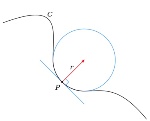
Parallel Transport (平行移動) 的定義
(Wiki 2019a) 微分幾何對平行移動的定義:
平行移動是將流形上的幾何特性沿著光滑曲線移動的一種方法。如果流形上有一個 affine connnection(covariant derivative),那麼 affine connection 保證我們可以將流形上的向量沿著曲線移動使得它們關於這個 connection 保持「平行」。
在某種意義上說,關於 connection 的平行移動提供了將流形的局部幾何沿著曲線移動的方法:即「連接」了鄰近點的幾何。有許多種平行移動的概念,但其中一種方式等同於提供了一個 connection。事實上,通常的 connection 是平行移動的無窮小類比。反之,平行移動是 connection 的局部實現。
因為平行移動給出了 connection 的一種局部實現,它也提供了曲率的一種局部實現(holonomy)。Ambrose-Singer 定理明確了曲率與 holonomy 的關係。

簡言之,平行移動基本是一種 local connection, 以及實現 curvature 的方式。
問題是:平行移動和平行公理有什麼關係?
平行公理和 Parallel Transport 和 geodesic 三角形內角和
平行公理:一條直線和線外一點平行直線的關係。
什麼是直線?最直觀的定義就是最短路徑,在非平面的“直線”看起來並不直。
數學的表示是: 
- 一條 Geodesics (地直線)上所有點的切向量(以及和切線固定夾角的向量)都互相平行(如下圖三條地直線,都是球面上的大圓)。
- Geodesic (地直線)線外一點和其最短距離的路徑也是 geodesic, 並且垂直夾角。
- 其實是否直角不重要。如果不是直角但仍是 geodesic,parallel transport 就會轉該夾角。沿著同一條 geodesic 的 parallel transport 和 geodesic 的夾角不變。
- How to prove? 如果 geodesic 構成的三角形內角和為 180, parallel transport 的夾角為 0. 大於 180, parallel transport 會產生正夾角。小於 180, parallel transport 產生負夾角。
平面和曲面幾何的 Parallel Transport (Holonomy)
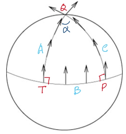
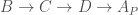
平面幾何:平行移動先定義 Geodesic A, 接著線外一點 P, 可以找到一條 Geodesic B 垂直於 A at T. 再來根據平行公理,只有一條平行線 Geodesic C 平行於 A, 且垂直於 B. 因為 A 和 C 是平行線,永不相交。為了讓 parallel transport 形成封閉迴路 (holonomy), 可以在 A 上找一點 Q, 並且做垂直線到 C, 稱為 geodesic D.
此時從 

柱面幾何:直接剖面切開就是平面。parallel transport 和平面一樣。如果沿著三角形 holonomy, 因為內角和為 180, 回到起點的 parallel transport 夾角為 0. Gauss curvature 為 0.
錐面幾何:圓錐面如下圖(a)的曲率?圓錐面可以展開成平面缺角圓形如下圖(b). 除了 A 點之外任何點的曲率為 0. 因為錐面上一個 close loop, 如果不包含 A, parallel transport 夾角為 0. 因此曲率為 0.
如果包含 A 的圓,parallel transport 夾角 = 


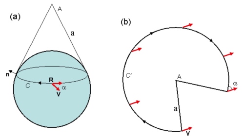
另一個問題,上圖球面非大圓 R 的 parallel transport 夾角? 常見的回答是 0. 錯誤的答案!正確的答案是用圓錐面和球面的切線為 R,再展開如上圖 b.
球面幾何:平行移動先定義 geodesic A (上圖左邊弧線), 赤道的 geodesic B 垂直於 A at T. 由平行定理我們知道球面幾何不存在和 A 平行(不相交)的 geodesic. 我們只能選擇和 B 垂直的 geodesic C, given we know A 和 C 會相交於 Q 點(其實在北極)。
此時從 


如果只是在局部做一個封閉迴路(holonomy),局部看起來就像歐氏空間。Parallel transport 的 holonomy 夾角為 0. Use Gauss curvature

雙曲線幾何:直接考慮鞍面的三角形,內角和小於 180. parallel transport 為負夾角。
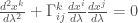
平行移動的數學表示
Parallel Transport 


Parallel transport 更數學而且和座標系無關的定義:

一個類比:如果不是一個向量 


平行移動和等高線的數學公式雖然非常類似。問題的形式 (formulation) 卻不同。
平行移動是給定一條任意線 

等高線是給定一個純量場
張量分析用於幾何
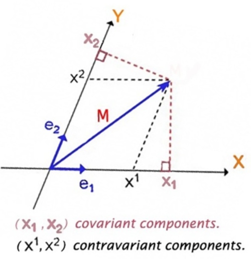
張量(tensor) 最重要的特性就是座標系無關,可用於平面或曲面。張量分為三類:
- Basis vector invariant: 純量 也就是 0 階張量。
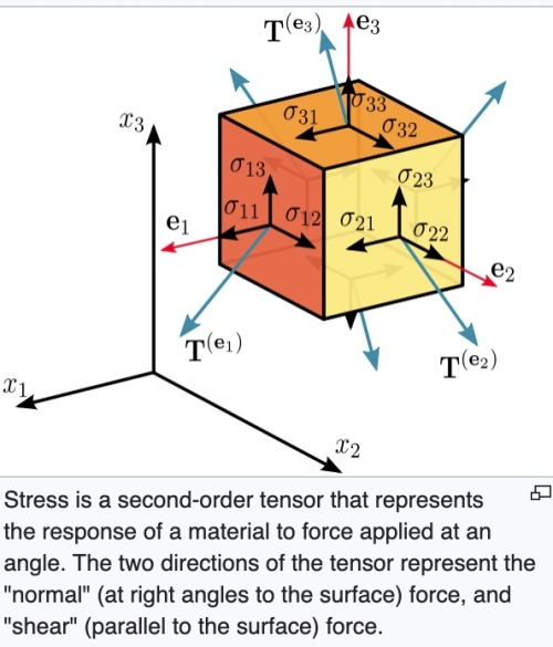
- Basis vector contra-variant. 為什麼 contra-variant? 因為 basis vector scale up, 張量分量會 scale down. 一階張量是 vector (n維), 二階張量 (nxn維), 三階張量(nxnxn維),依此類推。e.g. Einstein curvature tensor 是四階張量(4x4x4x4)維。 Ricci curvature tensor 是二階張量 (4×4)維。
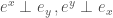
- Basis vector co-variant. 也稱為 one-form. 像是 gradient,
, basis vector scale up, dual basis vector scale down, 張量分量也會 scale up. 其他特性和一般張量一樣。
其他的張量運算下面展開。
先用歐氏空間的方向導數為例:
在卡氏座標系(笛卡爾直角座標系):
曲線和切向量:

注意:千萬不要用 ![[u_1, u_2]](https://s0.wp.com/latex.php?latex=%5Bu_1%2C+u_2%5D+&bg=fff&fg=444444&s=0&c=20201002)
先考慮 gradient operator,

一個純量場(0階張量)的梯度, 
一個一維量場的梯度, 
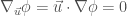
純量場的方向導數,基本上是純量場的梯度 (gradient) 和方向向量的內積。

(1) 只能用於卡氏座標系。接下來幾個重點:1.座標系無關;2.推廣到曲面;3.簡化公式。
現在引入 covariant/contravariant basis and tensor, 和愛因斯坦 summation notation.
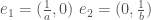
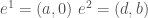
Basis vectors
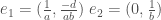
Dual basis vectors 

注意 


對於歐氏空間非直角座標系,(1) 可以修改為:

使用愛因斯坦 notation 重寫 (4)

曲面空間的方向導數:
曲面空間的純量場方向導數和 (5) 完全相同。因為純量場是 basis invariant.
但是曲面空間的向量場是 basis covariant or contravariant, 所以曲面的向量場的方向導數會比歐氏空間複雜的多。
曲面空間向量場
- 似乎可視每個分量為純量場,求每個純量場的方向導數。Wrong! 原因是 basis vector 在非歐空間不是 constant vector, 甚至歐氏空間的極座標也不是 constant vector. 因此 basis vector 的微分會產生新的 component! (Christopher symbol, or connection).
- 向量場的梯度是二階張量,直接求梯度太複雜。比較好的作法是分解方向導數的“方向向量”為 basis vector linear combination, 最後再結合為真正方向導數。
$latex \vec{V} = V^1 \mathbf{e_1} + V^2 \mathbf{e_2}
= V^{\alpha} \mathbf{e_\alpha} \\
\vec{u} = u^1 \mathbf{e_1} + u^2 \mathbf{e_2} $
$latex \nabla_{\vec{u}}\vec{V} = \vec{u}\cdot\nabla\vec{V}
= (u^1 \mathbf{e_1} + u^2 \mathbf{e_2})\cdot\nabla\vec{V} \\
\nabla_{e_\beta}\vec{V}=\mathbf{e_\beta} \cdot\nabla\vec{V}
= \mathbf{e_\beta} \cdot\nabla (V^\alpha \mathbf{e_\alpha})
= \mathbf{e_\beta} \cdot \frac{\partial(V^\alpha \mathbf{e_\alpha})}{\partial e_i} \mathbf{e^i} \\
= \frac{\partial(V^\alpha \mathbf{e_\alpha})}{\partial e_\beta}
= \frac{\partial V^\alpha}{\partial e_\beta}\mathbf{e_\alpha} +
V^\alpha \frac{\partial \mathbf{e_\alpha}}{\partial e_\beta}
= \frac{\partial V^\alpha}{\partial e_\beta}\mathbf{e_\alpha} +
V^\alpha \Gamma^k_{\alpha\beta}\mathbf{e_k} \\
= \frac{\partial V^\alpha}{\partial e_\beta}\mathbf{e_\alpha} +
V^i \Gamma^{\alpha}_{i\beta}\mathbf{e_\alpha}
= (\frac{\partial V^\alpha}{\partial e_\beta} +
V^i \Gamma^{\alpha}_{i\beta})\mathbf{e_\alpha} $
此處利用 Christopher symbol 以及
$latex \frac{\partial \mathbf{e_\alpha}}{\partial e_\beta} =
\Gamma^k_{\alpha\beta}\mathbf{e_k} $
如果是歐氏空間且直角座標系,Christopher symbol
如果是歐氏空間但極座標系,因為每一點的 local basis vector 方向都不同,Christopher symbol 不為 0, 一共有 2x2x2=8 個 components [@cyrilChristoffelSymbol2016].


愛因斯坦 notation and convention: 向量場的梯度微分是二階張量(樓上加樓下)。

最後 $latex \nabla_{\vec{u}}\vec{V} = \vec{u}\cdot\nabla\vec{V}
= (u^1 \mathbf{e_1} + u^2 \mathbf{e_2})\cdot\nabla\vec{V}\\
= u^\beta (\frac{\partial V^\alpha}{\partial e_\beta} +
V^i \Gamma^{\alpha}_{i\beta})\mathbf{e_\alpha}
= (u^i \frac{\partial V^k}{\partial e_i} +
u^i V^j \Gamma^{k}_{ij})\mathbf{e_k}
= (u^i {\partial_i V^k} +
u^i V^j \Gamma^{k}_{ij})\mathbf{e_k} $
愛因斯坦 notation and convention: 向量場的方向導數是一階張量(樓上)。
整理愛因斯坦 notation 的原則:
, 只有一個樓上 index,代表一階張量 contra-variant.
, 只有一個樓下 index,代表一階張量 co-variant (one-form).
, 張量和 1-form 張量內積結合,同一個 index i 樓上樓下抵銷,變成 0 階張量(純量)。
- 張量微分(gradient) 階數+1:
是二階(樓上加樓下)tensor.
- 張量和 one-form 張量內積 階數-1,index 樓上樓下抵銷。
- 張量場的方向導數是先微分張量(+1)場再和方向向量內積(-1),階數不變,e.g. 純量場方向導數是純量。向量場的方向導數是一階張量:
是一階(樓上) 張量。
- 因為張量場的方向導數階數不變。因此可以重覆這個運算。最常見是二次方向導數(沿不同的方向,如 basis vectors)。除了在平面歐氏座標系以外,一般是不能交換。
. 事實上,
? (TBC)
回到曲線的方向導數=絕對導數(Absolute Derivative:等高線,地直線,平行移動)
曲線和切向量回顧:
純量場的線方向導數
其實這就是著名的 gradient theorem, 或是線積分基本定理推廣到曲面。重點是曲面線積分是路徑無關!或是封閉迴路線積分為 0. 但在向量場不是如此。
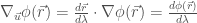
$latex \int_p^q \nabla_{\vec{u}}\phi(\vec{r}) d\lambda
= \int_p^q \nabla\phi(\vec{r})\cdot d\vec{r} = \phi(q) – \phi(p) $
以純量場為例
Let 
射線運動卡氏座標系:


射線運動極座標系:


以向量場為例
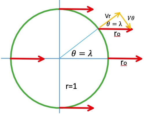
向量場的線方向導數,稱為絕對導數(absolute derivative)
$latex \nabla_{\vec{u}}\vec{V}(\vec{r}) = \frac{d\vec{r}}{d\lambda}\cdot\nabla\vec{V}(\vec{r}) \\
= u^i {\partial_i V^k} + u^i V^j \Gamma^{k}_{ij}
= \frac{d V^k}{d\lambda} + \frac{d x^i}{d\lambda} V^j \Gamma^{k}_{ij} $
Parallel transport


積分形式: 


另一個重點是 

卡氏座標系:

極座標系:


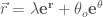
Example 1: 射線運動 (起點在r=1上)
Let 


Example 2: 圓周運動
Let 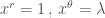


平行移動和曲率的關係
Geodesics 是 parallel transport 的特例


Reference
Gray, A., and L. Vanhecke. 1979. “Riemannian Geometry as Determined by
the Volumes of Small Geodesic Balls.” Acta Mathematica 142: 157–98.
https://doi.org/10.1007/BF02395060.
Keng, Brian. 2018. “Hyperbolic Geometry and Poincaré Embeddings.”
Bounded Rationality. June 17, 2018.
http://bjlkeng.github.io/posts/hyperbolic-geometry-and-poincare-embeddings/.
Wiki. 2019a. “Gaussian Curvature.” Wikipedia.
https://en.wikipedia.org/w/index.php?title=Gaussian_curvature&oldid=910677726.
———. 2019b. “Parallel Transport.” Wikipedia.
https://en.wikipedia.org/w/index.php?title=Parallel_transport&oldid=911069387.
———. 2019c. “Theorema Egregium.” Wikipedia.
https://en.wikipedia.org/w/index.php?title=Theorema_Egregium&oldid=895212511.

 -axis), 從下到上代表過去到未來。任何運動都可以用一條靜態的世界線(worldline) 表示。
 移動的觀察者。B 要如何得到 S 的 world line?
  (assuming
  ). 兩個不同的直角座標系 for S 運動,對應 A 和 B 觀察者 (observer oriented)。這不是我們所要的。如果有無窮多觀察者(等速或等加速觀察者)就需要無窮多直角座標系以及無窮多的 world lines for the same S 的運動。
 , 網格線 (grid line) 是正方形。但對 B 觀察者(相對速度為
  , 網格線是平行四邊形。此處是用 Lorentz 變換,所以
  格線是斜線。如果是 Galilean 變換,
 垂直線。對 B 座標系
  而言,
而言,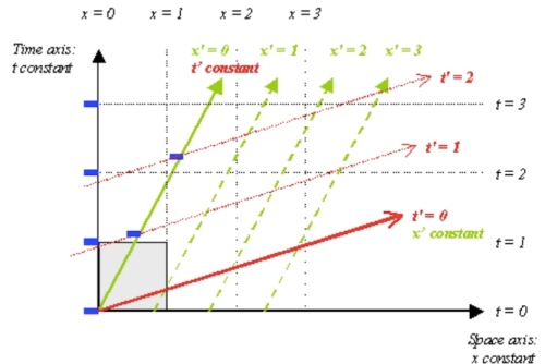
 網格線。下圖是 Lorentz 變換 C 的座標系。
  變成雙曲線。
 變成聚集在
變成聚集在  的投射線 (假設光速=1). 網格線變成更奇怪的四邊形。注意在 Lorentz transform 所有速度無法超越光速。觀察者 C 無法持續加速超越光速。 Galilean 變換 C 的座標系則不同。
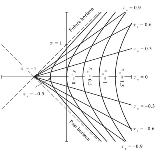
 幾何的一條世界線 C (不是面或其他形狀)
 幾何量是微分弧長 coordinate invariant 對應物理的 Lorentz transform. 如果少了
  就是 (-1)*Galilean transform.
 在 Galilean transform 不變。因為是 vector, vector components 在不同座標系不同,稱為 covariant. 對應的幾何不變量是“curvature vector". 但在 Lorentz transform,
  甚至不是 4-vector/tensor, 連 covariant 也不是。如何得到符合 Lorentz tranform 4-vector/tensor 的力學定律呢?下面描述。
 (單位是能量),differential action
  (單位是能量*時間,大自然兩者都要省)。Total action 就是空間兩點
  和時間兩點
和時間兩點  路徑積分。最小作用原理用變分法找到最小
  的路徑。
的路徑。 
 and
and  . 因為時間
  , 需要用 dummy variable
 沒有單位。根號的單位是速度,和光速
  單位抵銷。
單位抵銷。 的單位是能量。所以
  是 1st fundmental form 的根號,或是微分弧長。滿足 Lorentz transform invariant. In a word,
  重點是 S (action) 對應的是 4D 時空兩點之間的總弧長 (with a proportional constant). 最小作用原理對應幾何量是兩點之間最短距離的弧線,稱為 geodesic (測地線或地直線) which is coordinate invariant. [@cyrilGeodesicEquation2018] 也就是說,不同慣性運動的觀察者的最小作用原理都是一樣。但如何推廣到非慣性觀察者?
 base vector
  變大,component
  變小。所以是 contra-variance.
 , base vector
  越大, component 也越大。
  ?
? )。
)。 
 and
and  contra-variance, 因為
  和
和  是反比的關係。

 ).
). and
and  covariance, 因為
  和
和 
 ?
? 和
和  ,可以得出
,可以得出  !
! . 同時 normalize
 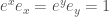 . 也就是反矩陣關係!
 除非
除非  是直角座標系。


 和
和  是反比。
是反比。 就愈小,稱為 contra-variance. 但是
  卻是愈大,和
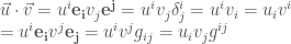
 斜角座標系
斜角座標系 


 的方向是由
的方向是由  所形成平面的法線 (normal) 決定,i.e.
  .
. 決定,i.e.
 所形成平面的法線 (normal) 決定。
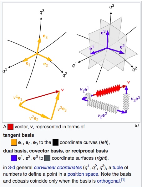


 metric tensor g matrix
 inverse metric tensor, 真的是 inverse g matrix.
 on orthonormal 座標系
 on 極座標系
 ,
,  ,
,  .
. ,
, 


 ,
, 
 :
:
 , 最小作用原理~?。

 座標系。為了簡化在 2D plan,只考慮
 替代
替代  . 一開始愛因斯坦並沒有 appreciate 閔式空間。閔式時空 (space-time) 引入微分幾何的觀念,為後來的廣義相對論開路。閔式空間和歐式空間一樣是平直空間。其微分第一基本式 (1st fundmental form)
  (平直空間 cross terms = 0)
  不滿足四維時空座標系不變,需要修正。
  和運動定律的慣性質量
  相等,
相等, or
or  . 也就是運動本身和球的特性(質量)無關。愛因斯坦認為這不是巧合,其中有非常深刻的意義。
 . 形式看起來一樣,但電磁力和慣性質量毫無關係。其他的各種力(磁力,弱力,核力)也都和慣性質量無關。這也是愛因斯坦時空場理論並不是另一個類似電磁場 Maxwell equations 的波動方程式。
  四維而且是四階張量。亦即一共有 4x4x4x4 = 256 個分量。相反質能只是一個純量。愛因斯坦面臨的問題是如何讓方程式兩邊能對接。也就是說:
 .
.

 是比例常數。