小米手機刷機
by allenlu2007
這是一個測試
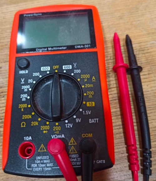
電池常見的困擾是到底有沒有電,還是裝置壞了。2020 我買了兩個東西非常有用。
三用電表: 主要用來量電壓,特別是電池電壓 (選 20V 檔位)。讓我了解不同裝置的操作電壓。
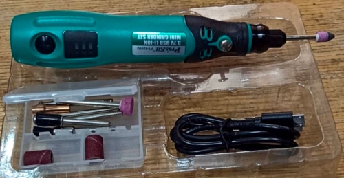
USB 充電磨砂機:幫我修理很多裝置生鏽造成接觸不良,而誤以為電池沒電。我買了下圖裝置,救了很多電器,非常有用。
AA/AAA/AAAA 電池的額定電壓是 1.5V.
這裡列出我用過的裝置單電池最低工作電壓。同時分為 A, B, C 三級,越低越優。
如果各位有測量裝置的最低工作電壓,請告訴我加入這個表。省錢兼環保!
| 廠牌 | 產品型號 | 電池 | failed電壓 | 級別 |
|---|---|---|---|---|
| 小米給皂機 | AA | 1.42V | C | |
| 美國給皂機 | AA | |||
| 羅技藍芽滑鼠 | M720 | AA | 1.36V | B |
| 日立冷氣遙控 | RF07T7 | AAA | 1.38V | B |
本文聚焦在 Ubuntu 16.04 LTS with GTX1080 GPU deep learning 軟體設定。
2021/3/28 加上 Ubuntu 20.04 LTS 的軟體設定在最後。
Reference:
[1] tflearn: http://tflearn.org/examples/
[2] https://standbymesss.blogspot.tw/2016/09/ubuntu-1404-caffe-cuda-75-opencv-31.html -> good reference
[bootable USB stick]
[3] “Create a bootable USB stick on Ubuntu“
[4] “Create a bootable USB stick on Windows (Rufus)”
Why Choose 16.04? Tensorflow/CUDA/Android Studio trade-off
* Use USB booting to install Ubuntu 16.04
If host is windows, use Rufus [4]. If host is Ubuntu, see [3].
* Choose Ubuntu 16.04 desktop version.
=> Check the update and 3rd party during the installation
=> use others option and choose mount point / and format the partition
After successful installing Ubuntu 16.04
* Setup -> software update —> additional driver —> GTX 1080 —> choose Nvidia driver xxx to install Nvidia driver instead of using Xorg driver.
這步似乎可以省略。之後 install CUDA10 會自動用 nvidia 最新的 driver.
$ sudo apt-get update
$ sudo apt-get upgrade
Reference: Linux MATLAB 2018a installation
$ sudo mkdir /mnt/matlab
$ sudo mount -o loop R2018a_glnxa64_dvd1.iso /mnt/matlab
$ cd /mnt/
$ sudo /mnt/matlab/install
等到安裝到 60% 會提示插入第二張 CD, 執行:
$ sudo mount -o loop R2018a_glnxa64_dvd2.iso /mnt/matlab
之後就 follow readme.txt 的 instruction.
Matlab 此時會使用 GTX 1080.
* sudo apt install emacs
* sudo apt install git
* vnc 可以參考下文。==> change to the following reference using ubuntu default desktop sharing!
=> use team viewer is better!!!
* Change locale 去除星期的中文字
ps. edit /etc/default/locale to change the date format from lzh_TW -> en_US.UTF-8
Reference:
1.2. ls /usr/localls : CUDA
1.3. http://docs.nvidia.com/deeplearning/sdk/cudnn-install/index.html:cudnn
Reference:
* CUDA 8.0 -> CUDA 10.1 (2019/3/1) -> CUDA 10.0 (3/8)
CUDA10.1 is too new to be compatible with tensor flow1.13!
Use CUDA10.0 instead
$nvcc —version (may need to do $sudo apt install nvidia-cuds-toolkit
$nvidia-smi

Setup environment variables
export CUDA_HOME=/usr/local/cuda-8.0
export LD_LIBRARY_PATH=${CUDA_HOME}/lib64
PATH=${CUDA_HOME}/bin:${PATH}
export PATH
* cuDNN: 6.0 -> 7.5 (2019/3/1)
sudo dpkg -i libcudnn7_7.0.2.43-1+cuda9.0_amd64.deb
sudo dpkg -i libcudnn7-dev_7.0.2.43-1+cuda9.0_amd64.deb
sudo dpkg -i libcudnn7-doc_7.0.2.43-1+cuda9.0_amd64.deb
注意在 install cuDNN 後,依照 Nvidia cuDNN installation guide (reference 3) compile mnistCUDNN example.
遇到以下錯誤。
Can not use cuDNN on context None: cannot compile with cuDNN. We got this error: In file included from /usr/local/cuda-8.0/include/channel_descriptor.h:62:0, from /usr/local/cuda-8.0/include/cuda_runtime.h:90, from /usr/include/cudnn.h:64, from /tmp/try_flags_F2eFMF.c:4: /usr/local/cuda-8.0/include/cuda_runtime_api.h:1628:101: error: use of enum 『cudaDeviceP2PAttr' without previous declaration extern __host__ __cudart_builtin__ cudaError_t CUDARTAPI cudaDeviceGetP2PAttribute(int *value, enum cudaDeviceP2PAttr attr, int srcDevice, int dstDevice); ^參考 https://github.com/Theano/Theano/issues/5856 解決這個問題。
Open the file:
/usr/include/cudnn.h
And try change the line:
#include “driver_types.h”
to:
#include <driver_types.h>
--------------------------------
在 2.3.1 installing from a Tar File.
Copy the following files into the CUDA Toolkit directory.
$ sudo cp cuda/include/cudnn.h /usr/local/cuda/include
$ sudo cp cuda/lib64/libcudnn* /usr/local/cuda/lib64
$ sudo chmod a+r /usr/local/cuda/include/cudnn.h /usr/local/cuda/lib64/libcudnn*
不過用 2.3.2 installing from a Debian File (as I did). 在以上目錄 (/usr/local/cuda/include and lib) 卻找不到 cudnn or libcudnn files.
反而是在 /usr/include/x86_64-linux-gnu/include and lib, why?

https://standbymesss.blogspot.tw/2016/09/ubuntu-1404-caffe-cuda-75-opencv-31.html
$ sudo apt-get install libprotobuf-dev libleveldb-dev libsnappy-dev libopencv-dev libhdf5-serial-dev protobuf-compiler
$ sudo apt-get install --no-install-recommends libboost-all-dev
$ sudo apt-get install libgflags-dev libgoogle-glog-dev liblmdb-dev
Install Atlas
$ sudo apt-get install libatlas-base-dev
Download anaconda2, use python 2.7.13 for caffe compatibility
$ bash Anaconda2-4.0.0-Linux-x86_64.sh
參考 https://standbymesss.blogspot.tw/2016/09/ubuntu-1404-caffe-cuda-75-opencv-31.html
$ sudo apt-get install cmake git libgtk2.0-dev pkg-config libavcodec-dev libavformat-dev libswscale-dev
$ unzip opencv-3.3.0.zip
$ cd opencv-3.1.0/ $ mkdir release $ cd release $ cmake -DBUILD_TIFF=ON -DENABLE_AVX=ON -DWITH_OPENGL=ON -DWITH_OPENCL=ON -DWITH_IPP=ON -DWITH_TBB=ON -DWITH_EIGEN=ON -DWITH_V4L=ON -DCMAKE_BUILD_TYPE=RELEASE -DCMAKE_INSTALL_PREFIX=$(python -c "import sys; print(sys.prefix)")-DPYTHON_EXECUTABLE=$(which python)-DPYTHON_INCLUDE_DIR=$(python -c "from distutils.sysconfig import get_python_inc; print(get_python_inc())")-DPYTHON_PACKAGES_PATH=$(python -c "from distutils.sysconfig import get_python_lib; print(get_python_lib())")..
$ make -j8
test opencv
a. run python and do “import cv2″
b. using ./python/python demo.py
我遇到問題是
GLib-GIO-Message:Using the 'memory'GSettings backend.export GIO_EXTRA_MODULES=/usr/lib/x86_64-linux-gnu/gio/modules/
git download caffe.
cd caffe directory.
$ cd python
$ for req in $(cat requirements.txt);do pip install $req;done
$ cd ..
$ cp Makefile.config.example Makefile.config
Modify Makefile.config based on the reference.
$make all -j8
$make test -j8
all OK
$make runtest -j8
encounter library libhdf5_hl_so.8 problem!!
Add ${ANACONDA2}/lib path to LD_LIBRARY_PATH to solve this problem.

pycaffe
make python
# for Ubuntu 16.04
sudo apt-get install -y --no-install-recommends libgflags-dev
# for both Ubuntu 14.04 and 16.04
sudo apt-get install -y --no-install-recommends \
      libgtest-dev \
      libiomp-dev \
      libleveldb-dev \
      liblmdb-dev \
      libopencv-dev \
      libopenmpi-dev \
      libsnappy-dev \
      openmpi-bin \
      openmpi-doc \
      python-pydot
sudo pip install \
      flask \
      future \
      graphviz \
      hypothesis \
      jupyter \
      matplotlib \
      pydot python-nvd3 \
      pyyaml \
      requests \
      scikit-image \
      scipy \
      setuptools \
      six \
      tornado
git clone –recursive https://github.com/caffe2/caffe2.git && cd caffe2
make &&cd build && sudo make install
python -c ‘from caffe2.python import core’ 2>/dev/null &&echo“Success”||echo“Failure”
python -m caffe2.python.operator_test.relu_op_test
https://blog.csdn.net/hgdwdtt/article/details/78633232
sudo apt-get install libcupti-dev
conda create -n tensorflow python=3.6
source activate tensorflow
Cuda-10.1 seems not supported by tensorflow-gpu.
Need to compile from source : difficult and not recommend
pip install —upgrade tensorflow-gpu
Got the following error message!!
_mod = imp.load_module(‘_pywrap_tensorflow_internal’, fp, pathname, description)
File “/home/alu/anaconda3/envs/tensorflow/lib/python3.6/imp.py”, line 243, in load_module
return load_dynamic(name, filename, file)
File “/home/alu/anaconda3/envs/tensorflow/lib/python3.6/imp.py”, line 343, in load_dynamic
return _load(spec)
ImportError: libcublas.so.10.0: cannot open shared object file: No such file or directory
Solve this problem by installing cuda10.0.!
Install Keras
Pip install keras
Install PytTorch
conda install pytorch torchvision cudatoolkit=10.0 -c pytorch
pip install mxnet-cu80==0.11.0
主要是用來 run mtcnn for face detection.
Step 5: install tflearn
pip install tflearn or condo install tflearn?
Step 6: install caffe/caffe2? to run faster R-CNN
Reference:
https://storage.googleapis.com/tensorflow/linux/gpu/tensorflow_gpu-1.3.0-cp27-none-linux_x86_64.whl
$ sudo mkdir /mnt/matlab$ sudo mount -o loop R2018a_glnxa64_dvd1.iso /mnt/matlab$ cd /mnt/$ sudo ./mnt/matlab/install
[1] Ubuntu 20.04 CUDA 11.1 cuDNN 8.0.4 install
[2] Create a bootable USB stick on Windows

Install Ubuntu 20.04 LTS
1. Create USB bootable drive using Rufus (windows) using the DataTraveler USB drive (32GB), [2]
2. 遵循上面 link 的指示,選擇 Ubuntu 20.04 LTS desktop iso 如下。

3.Boot from USB and do the installation.
Referece
[1] https://jianjiesun.medium.com/ubuntu-20-04-cuda-11-1-cudnn-8-0-4-install-62b7fe24941d. Errors for copy cudnn!!! Use the following!!!
Or
[2] https://docs.nvidia.com/deeplearning/cudnn/install-guide/index.html
實際和 [1] 有幾點不同:
1. Driver installation 很難搞。最後成功把 nvidia 官網download 455 driver installed. 但忘記如何搞定。 Do “$nvidia-smi -l” to check the driver installation.
2. 在 install CUDA11.1, 記得 bypass install driver (x blank). Do “$make all”; in the $NVIDIA_CUDA-11.1_Sample directory to check CUDA installation.
3. Install cudnn [1] and [2]
Method1:
直接 include and lib. 但是 path 如下:
$ sudo cp cuda/include/cudnn*.h /usr/local/cuda/include
$ sudo cp -p cuda/lib64/libcudnn* /usr/local/cuda/lib64
$ sudo chmod a+r /usr/local/cuda/include/cudnn*.h /usr/local/cuda/lib64/libcudnn*
Method 2:
Use deb dpkg to install (i) libcudnn; (ii) dev; (iii) sample code;
$ sudo
dpkg -i libcu sudo dpkg -i libcudnn8-dev_8.x.x.x-1+cudax.x_amd64.deb
$ sudo dpkg -i libcudnn8-dev_8.x.x.x-1+cudax.x_amd64.deb
$ sudo dpkg -i libcudnn8-samples_8.x.x.x-1+cudax.x_amd64.deb
Method2 seems to be easier, especially for sample code. 不過我先用 method1,就沒有用 method2。
4. Verify Install cudnn [2]
Copy the cuDNN samples to a writable path.
$cp -r /usr/src/cudnn_samples_v8/ $HOME
Go to the writable path.
$ cd $HOME/cudnn_samples_v8/mnistCUDNN
Compile the mnistCUDNN sample.
$sudo apt-get install libfreeimage3 libfreeimage-dev
$make clean && make
Run the mnistCUDNN sample.
$ ./mnistCUDNN
If cuDNN is properly installed and running on your Linux system, you will see a message similar to the following:
Test passed!
為了 check cudnn install, 我從 sda6 copy /usr/src/cudnn_sample code to verify.
Install Anaconda, create virtual environment, 安裝pytorch and常見套件
1. Download anaconda and “$ bash
Anaconda3-2020.11-Linux-x86_64.sh” to install anaconda
2. Create a virtual environment using conda with python 3.6
$ conda create –name torch36 python=3.6
$ conda activate torch36
3. 把 source activate torch36 加入 .bashrc, 重開 terminal to install pytorch. 到 pytorch 官網選擇 ubuntu, cuda=11.1, …
$ conda install pytorch torchvision
torchaudio cudatoolkit=11.1 -c pytorch -c conda-forge
4.
$ conda install matplotlib,pandas, jupyter, jupterlab… 安裝常用的套件。我產生一個 torch36.yml. 只要 $ conda env create -f torch36.yml
Install other software 常用的 software 如 emacs, git, kdiff3, teamviewer, dropbox.
Emacs: $sudo apt install emacs
Git: $ sudo apt install git
Kdiff3: $ sudo apt install kdiff3
Teamviewer:
$ sudo apt update
$ sudo apt install gdebi-core wget
$ wget https://download.teamviewer.com/download/linux/teamviewer_amd64.deb
$ sudo apt install ./teamviewer_amd64.deb
$ teamviewer => run teamviewer
Dropbox: 直接在 Application search dropbox
(not caje dropbox) and install
Install huggingFace transformer
可以用 pip or conda, https://github.com/huggingface/transformers
Pip:
$ pip install transformers
Conda:
$ conda install -c huggingface transformers
我用 conda to install huggingface
transformers.
虛擬化無處不在。1998 VMware 成立標誌 virtual machine (VM) 正式進入商業化。可以說 VM enable 之後的 cloud 服務 例如 Amazon/AWS, Microsoft/Azure, Google/GCP. VM 讓有限的 servers 分身成 virtual machines 服務數百或數千倍的使用者,儘量 exploit multiple user 的 statistical multiplexing gain. 同時藉著 virtual machine configuration 提供差異化的服務和收費。
VM 當然不只是用於 cloud 服務, 也可以用於 edge machine or device. 其實 VMware 的初衷是用於 edge or terminal device, 畢竟當時還沒有 cloud 服務. 不過在一台 computer install 多個 VMs 似乎只是少數 geeks or nerds 的嗜好,並非一般人的需要。
倒是一個新的趨勢是跨平台的應用需要類似 "virtual machine" on edge machine or device. 舉個例子,在 Windows/Mac/Linux 的平台可以 run NAS/BT/Wordpress 服務, 或是 AI framework and application. 我們需要跨系統平台 (Windows/Mac/Linux) App 執行不同的服務. 這些 App 大多是 linux-base. 但 linux 本身也是極端 fragmented, 不同的 distribution (Ubuntu/CentOS/Redhat/Debian/…) 以及不同的版本。因此類似 “application virtual machine" 可以自由運行在不同平台就非常方便 deploy service.
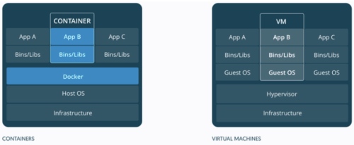
Virtual machine 一個主要問題是太佔系統資源,需要完整的 Guest OS, Bins/Libs, 如上圖右。一台 computer 可能只能運行兩三個 virtual machine. Docker 因此應運而生如上圖左。Docker 上的 container 類似 VM, 但輕薄很多,只有必要的 Bins/Libs. 下圖的卡通生動的描述:鯨魚就是 Docker, 一個 docker 可以有很多的貨櫃 (container), 每一個 container 可以視為是 light weight virtual machine. 一個 docker 可以運行多個,甚至十數個 light weight container of services. 此外,一部 computer 也可以運行多個 docker. 但一般只運行一個 docker 管理多個 containers.
Virtual machines 和 containers 都是在同一個 host computer 分享相同的資源, e.g. CPU, GPU, Memory, etc. Docker and container 通常用於一般 服務, 因為 containers 之間的隔離性和保密性比 virtual machine 差。Virtual machine 對於需要高度保密服務,例如 payment, copyright, 生物特徵仍然有必要。例如手機一般會用 TEE (Trusted Execution Environment) on Hypervisor 處理 payment 或是 finger print 或是 face ID 的資訊。 TEE 可以視為一種 VM (light weight on light OS).
VM vs. docker container 有點像 process vs. thread in a multi-task OS. Process 之間都是隔離和獨立。 Thread 之間可以是合作關係甚至分享資源。
本文聚集在 docker. 我們跳脫一般從抽象的 command line docker 入手,直接從 portainer dashboard 介紹 docker 的運行。
Portainer 本身就是一個 container, 具有以下的特性:
先假設 docker 和 portainer 已經安裝好,例如使用 OpenMediaVault for NAS solution.
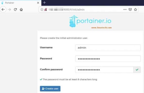
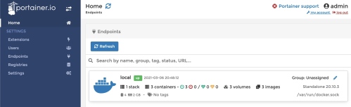
Step 1: 第一次啟動 portainer 需要設定 Username and Password 如下:
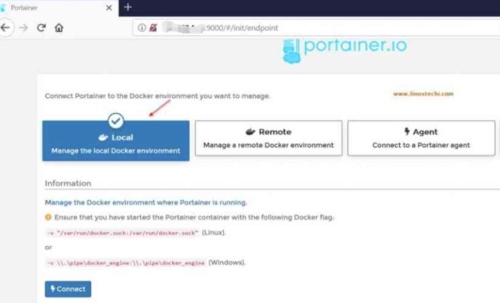
Step 2: 如果是在 docker 的 host 安裝 portainer (in this case), 選擇 local docker.
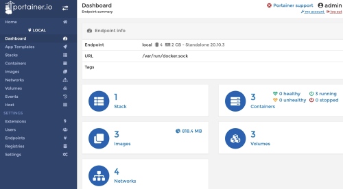
Step 3: 此時顯示 local docker 的 summary information. 包含 (1) stack; (3) containers; (3) volumes; (3) images.
Step 4: 點擊任一項目 (stack/container/volume/image) 進入 Dashboard (Endpoint summary), 就是下圖左 panel 第一項,右邊內容和上圖一樣。
我們逐一解釋 panel 的項目,藉此了解 docker 的運作。
選擇左邊 panel 的 container. 這是 docker 核心功能。這裡看到有 3 個 containers. 從 Container Name 可以粗略判斷提供什麼服務。例如中間 container 就是 portainer 本身,提供 docker 管理服務。其他兩個是我之前執行的 wordpress 和 qbittorrent 兩個 containers 提供 blog 和 BT 服務。
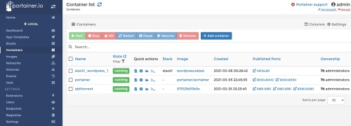
Status: 可以 start/stop/kill/… 這個 container (service).
Image: 代表這個 container 是由該 image 創造出來的。一個 image 可以創造出多個不同的 containers. 另外 image 是 Read-Only 無法改變內部的設置,例如 library, module, etc. 只有在創建 container, image 會被包覆在一層 "think R/W layer" 之下。通過這層 layer 才可以改變 container 內部的設置。
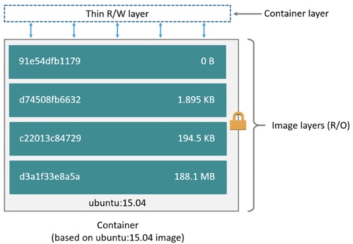
Image 和 container 的關係,相當於與 OOP 中 class and object 的關係。
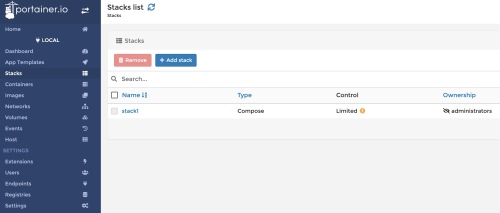
Stack: Optional. 後面再討論。
Ports: 相反是 container 開放給外部的 service 或是 access. 注意有兩個 port number, 一個對應 container 內部的 port number, 另一個對應外部 access container 的 port number, 一般相同,但不需要一樣。
Created and Ownership 很直觀不用說明。
我們後面用實例討論如何 Add container.
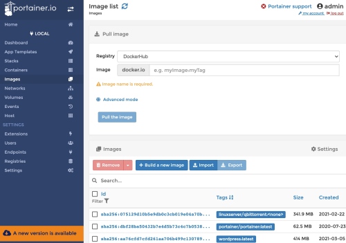
選擇左邊 panel 的 image. 先看右下半 Images 部分,代表 docker 所有的 images. Containers 就是從 images 創造出來,所以 image created 日期一定早於 container crated 日期。 Image 一般是從 Registry pull 來的,就是右上半 Pull image 部分。最普遍的 registry 是 DockerHub? 可以到 DockerHub (project 之於 github 類似 image 之於 DockerHub) search images https://hub.docker.com. 常用的 image 包含各類的 linux distributions 以及各種 service or database. Image 可以被 remove/import/export/…
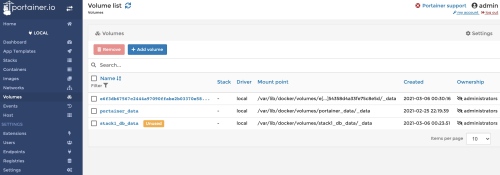
Volume 是 docker 存放 data 的地方。選擇左邊 panel 的 volume.
其中有 3 個 volume, 從 Name 就可以判斷中間的 volume 是 portainer 存放 data 的 directory. Mounting point 是對應 host 的絕對路徑。
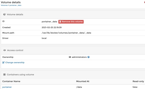
點擊 portainer_data volume 可以得到更明確的資訊:前面的部分都一樣。最後有對應的 Container Name.
By default 所有在 container 中建立的檔案都儲存在 container thin R/W layer 上,這表示:
因此必須有其他的機制,將 container 中的檔案留存在 host 上,Docker 有兩種作法:volume 和 bind mount. 另外在 Linux 作業系統上的 Docker 還可使用 tmpfs mount (暫存)。這三種方式的差異可用下圖表示。
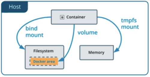
這三者的差異:
Volume 是 Docker 最推薦存放 persisting data 的機制,使用 Volume 有下列優點
Stack 不是傳統資料結構的 stack,而是 “stack" 不同的 images 構成完整的 container 可以提供完整的 service. 要建立一個可提供應用程式完整執行環境的 Container image,要先從一個 Base Image (例如 Ubuntu OS) 開始疊起,一層層將不同 Stack 的 image 疊加上去,最後組合成一個應用程式所需Container 執行環境的 image, 如下圖。
一個Stack就是一層Container image
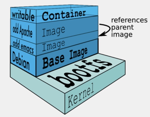
舉例來說,假設一個網頁執行環境需要有OS、Apache網站伺服器、MySQL資料庫、Ruby執行環境等不同的Stack。
最常用的基礎映象檔就是ubuntu映象檔,這是用來建立Container的根目錄架構,若採用了不同的OS映象檔,就會變成是那個OS的目錄架構。
第一個動作就是先 pull the ubuntu 的基礎 image: 只要在命令列輸入sudo docker pull ubuntu,預設pull指令都是存取Docker Hub服務。這個指令會從Docker Hub上下載名稱為ubuntu的 image 到本機端。
接著,要將新的一層Stack加入ubuntu基礎映象檔中,例如Apache,得先用Docker執行(Docker run指令)這個基礎 image,來建立這個 image 的Container,然後在Container中安裝Apache,安裝完成後,再將Container打包成另一個新的 image。
第二層繼續反覆這樣的程序,這時候就是直接從ubuntu-Apache所建立的 image 開始安裝下一層的MySQL程式,同樣也是先執行ubuntu image,再執行MySQL安裝程序。
說來複雜,實際執行過程,執行映象檔和安裝Apache是一行指令,命令Docker從ubuntu映象檔來建立新的Container同時在這個Container內執行Apache安裝指令。
當Apache安裝完成後,Container的壽命也跟著結束了,除非是Daemon式的背景程式,那麼這個Container才會一直存活。就算只是在Container裡面執行一個ls(列出目錄架構)的指令,如sudo docker run ubuntu ls -1。Container也是在ls–l指令結束後也同時關閉了。一行指令就建立了一次Container,也關閉了這個Container。
Reference
[1] Dennis TS, Medium, “使用Docker來建置Deep Learning環境”.
[2] 蝈蝈, 知乎, “Docker,救你于「深度学习环境配置」的苦海”.
[3] twtrubiks, github, https://github.com/twtrubiks/docker-tutorial
[4] Docker, “Dcoker Desktop for Mac“
過去都是使用anaconda+tensorflow+keras+pytorch 來開發Deep Learning,但時間久了會發現直接安裝的cuda與cudnn的更新相當麻煩,久了也難以管理,因此學習使用Docker來建立Deep Learning環境,大部分的步驟都與官網的說明相同,這篇文章就是建置過程的一個紀錄。
ubuntu 16.04

先了解一下 Docker 中的幾個名詞,分別為
Image
映像檔,可以把它想成是以前我們在玩 VM 的 Guest OS( 安裝在虛擬機上的作業系統 )。
Image 是唯讀( R\O )
Container
容器,利用映像檔( Image )所創造出來的,一個 Image 可以創造出多個不同的 Container,
Container 也可以被啟動、開始、停止、刪除,並且互相分離。
Container 在啟動的時候會建立一層在最外(上)層並且是讀寫模式( R\W )。
這張圖解釋了 Image 是唯讀( R\O )以及 Container 是讀寫模式( R\W ) 的關係

Image 是一个个配置好的环境。 container 是image的具体实例。 image 和 container 的关系,相当于与 class and object 的關係。
Registry
可以把它想成類似 GitHub,裡面存放了非常多的 Image ,可在 Docker Hub 中查看。
參考 https://docs.docker.com/install/linux/docker-ce/ubuntu/
$ sudo apt-get update
$ sudo apt-get install \
apt-transport-https \
ca-certificates \
curl \
gnupg-agent \
software-properties-common
$ curl -fsSL https://download.docker.com/linux/ubuntu/gpg | sudo apt-key add –
$ sudo add-apt-repository \
“deb [arch=amd64] https://download.docker.com/linux/ubuntu \
$(lsb_release -cs) \
stable”
$ sudo apt-get update
$ sudo apt-get install docker-ce docker-ce-cli containerd.io
To verify:
$ sudo docker run hello-world
一般來說,若只是要使用虛擬環境,只要安裝完Docker就好了,但若是要開發Deep Learning應用,就必須使用到GPU,而nvidia-docker就是docker的一個包裝,他可以輕易的讓你的虛擬環境使用GPU。安裝程序也是參照官網。
加入金鑰
$ curl -s -L https://nvidia.github.io/nvidia-docker/gpgkey | \
$ sudo apt-key add –
2. 加入 repository
# Add the package repositories
$ distribution=$(. /etc/os-release;echo $ID$VERSION_ID)
$ curl -s -L https://nvidia.github.io/nvidia-docker/gpgkey | sudo apt-key add –
$ curl -s -L https://nvidia.github.io/nvidia-docker/$distribution/nvidia-docker.list | sudo tee /etc/apt/sources.list.d/nvidia-docker.list
$ sudo apt-get update && sudo apt-get install -y nvidia-container-toolkit
$ sudo systemctl restart docker
此時 docker = nvidia-docker, check by
$ sudo docker –version
$ sudo nvidia-docker –version
All the same:
Docker version 19.03.7, build 7141c199a2
6. 用CUDA image來作測試
#### Test nvidia-smi with the latest official CUDA image
$ sudo docker run –gpus all nvidia/cuda:10.0-base nvidia-smi
Deepo 是一個含有許多Deep Learning Framework的docker image,使用這個image,可以讓我們快速的建置一個虛擬環境。
If use old version (10.0), if 10.1 version ignoring the :py36-cu100
$ sudo docker pull ufoym/deepo:py36-cu100
Install jupyter
$ sudo docker pull ufoym/deepo:all-jupyter-py36-cu100
Test the nvidia-smi in deepo
$ sudo docker run –gpus all –rm ufoym/deepo:py36-cu100 nvidia-smi ## —rm means remove container after exit
Create a bash of the nvidia/deepo docker
$ sudo docker run –gpus all -it ufoym/deepo:py36-cu100 bash
$ ctl-d # to quit the bash
Create a bash of the nvidia/deepo docker 並 mount host directory to docker (-v)
$ sudo docker run –gpus all -it -v /host/data:/data -v /hsot/config:/config ufoym/deepo:py36-cu100 bash
Create a bash of the nvidia/deepo docker and check the framework is installed and version
$ python
>>> import tensorflow
>>> import sonnet (AttributeError: module ‘tensorflow’ has no attribute ‘GraphKeys’)
>>> import torch
>>> import keras (no need for tensorflow2)
>>> import mxnet
>>> import cntk
>>> import chainer
>>> import lasagne
>>> import caffe
>>> import caffe2
Use pip list to check the framework version
$ pip list
mxnet-cu100 1.5.1.post0
tensorflow-estimator-2.0-preview 2.0.0
tensorflow-probability 0.8.0
termcolor 1.1.0
tf-nightly-gpu-2.0-preview 2.0.0.dev20191002 (tensorflow 2.0)
Theano 1.0.4+unknown
torch 1.3.0 (pytorch 1.3)
torch-nightly 1.2.0.dev20190805 (why nightly 1.2.0?)
torchvision 0.5.0a0+1e857d9
Keras 2.3.1
Keras-Applications 1.0.8
Keras-Preprocessing 1.1.0
mxnet-cu100 1.5.1.post0
mxnet-cu100 1.5.1.post0
Lasagne 0.2.dev1
$ caffe —version
caffe version 1.0.0
$ darknet
$ th (for torch 7) => deprecated, no use.
It seems to have lots of problems.
1. Pytorch:
Issue: File “/usr/local/lib/python3.6/dist-packages/torchvision/models/inception.py”, line 168, in Inception3
@torch.jit.unused
AttributeError: module ‘torch.jit’ has no attribute ‘unused’
2. Tensorflow (2.0)
Issue: File “mnist.py”, line 15, in from tensorflow.examples.tutorials.mnist import input_data ModuleNotFoundError: No module named ‘tensorflow.examples.tutorials’
Check docker version
$ sudo docker –version
Docker version 19.03.7, build 7141c199a2
Check docker image
$ sudo docker images
REPOSITORY TAG IMAGE ID CREATED SIZE
ufoym/deepo latest 69b30aa9ad32 5 weeks ago 12.8GB
nvidia/cuda latest 9e47e9dfcb9a 3 months ago 2.83GB
nvidia/cuda 10.0-base 841d44dd4b3c 3 months ago 110MB
nvidia/cuda 10.1-base 3b55548ae91f 3 months ago 106MB
ufoym/deepo py36-cu100 394b64d11e28 4 months ago 10.9GB
ufoym/deepo all-jupyter-py36-cu100 cf60a305ba7b 6 months ago 10.9GB
hello-world latest fce289e99eb9 14 months ago 1.84kB
建立 image (類似 git)
$ sudo docker create -it –name busybox busybox
or use docker pull
$ sudo docker pull ufoym/deepo:all-jupyter-py36-cu100
刪除 Image
$ docker rmi [OPTIONS] IMAGE [IMAGE…]
查看目前運行的 container
$ docker ps
查看目前全部的 container( 包含停止狀態的 container )
$ docker ps -a
新建並啟動 Container (docker run)
docker run [-it] some-image 创建某个镜像的容器。注意,同一个镜像可以通过这种方式创建任意多个container. 加上-it之后,可以创建之后,马上进入交互模式。
$ docker run [OPTIONS] IMAGE[:TAG|@DIGEST] [COMMAND] [ARG…]
如何查询命令参数: docker可以看docker客户端有那些基本命令; 对应每一条命令,想看看具体是做什么的,可以在后面加一个 –help查看具体用法,例如对于run命令: docker run –help
$ docker run –gpus all nvidia/cuda:10.0-base nvidia-smi
$ docker run –gpus all -it ufoym/deepo:py36-cu100 bash ## -it means interactive; —rm means quit container after exit
$ docker ps -a ## list all containers
$ docker rm container-id ## docker rmi image
退出 container
ctl-d or exit to quit container. ctl-q-p exit but container is running.
接下來要介紹 Volume,Volume 是 Docker 最推薦存放 persisting data( 數據 )的機制,
使用 Volume 有下列優點
Volumes are easier to back up or migrate than bind mounts.
You can manage volumes using Docker CLI commands or the Docker API.
Volumes work on both Linux and Windows containers.
Volumes can be more safely shared among multiple containers.
Volume drivers allow you to store volumes on remote hosts or cloud providers, to encrypt the contents of volumes, or to add other functionality.
A new volume’s contents can be pre-populated by a container.
在 container 的可寫層中,使用 volume 是一個比較好的選擇,因為他不會增加 container 的容量,
volume 的內容存在於 container 之外。

建議大家花點時間研究 docker 中的 network,會蠻有幫助的 😃
查看目前 docker 的網路清單
docker network ls [OPTIONS]
詳細可參考 https://docs.docker.com/engine/userguide/networking/
docker 中的網路主要有三種 Bridge、Host、None,預設皆為 Bridge 模式。
$ sudo docker volume create portainer_data
$ docker run –name=portainer -d -p 9000:9000 -v /var/run/docker.sock:/var/run/docker.sock -v portainer_data:/data portainer/portainer
reference: https://github.com/twtrubiks/docker-tutorial#volume
$ sudo docker run -it ufoym/deepo:all-jupyter-py36-cu100 bash
2 containers: ufoym/deepo…..-cu100; and portainer

2 images: ufoym/deepo….-cu100; and portaner:latest

Since no —rm, after ctl-d, container becomes:

image is the same.
After I remove the stopped container and do
$ sudo docker run -it —rm ufoym/deepo:all-jupyter-py36-cu100 bash
same as before, after ctl-d container becomes:

1. create a container for remote visit
$ sudo nvidia-docker run -it -p 7777:8888 –ipc=host -v /home/alu/Documents/gby:/gby –name gby-notebook ufoym/deepo:all-jupyter-py36-cu100
Container and image.


2. Start jupyter notebook after creating a container
$ jupyter notebook –no-browser –ip=0.0.0.0 –allow-root –NotebookApp.token= –notebook-dir=’/gby’
3. Local host do:
Step1: get docker.dmg from https://hub.docker.com/editions/community/docker-ce-desktop-mac/
Step2: run docker.dmg and the status bar shows:

Step3: open a terminal and run: docker version =>
(tf) Allende-MBP:cheers2019 allenlu$ docker version
Client: Docker Engine – Community
Version: 19.03.8
API version: 1.40
Go version: go1.12.17
Git commit: afacb8b
Built: Wed Mar 11 01:21:11 2020
OS/Arch: darwin/amd64
Experimental: false
Server: Docker Engine – Community
Engine:
Version: 19.03.8
API version: 1.40 (minimum version 1.12)
Go version: go1.12.17
Git commit: afacb8b
Built: Wed Mar 11 01:29:16 2020
OS/Arch: linux/amd64
Experimental: false
containerd:
Version: v1.2.13
GitCommit: 7ad184331fa3e55e52b890ea95e65ba581ae3429
runc:
Version: 1.0.0-rc10
GitCommit: dc9208a3303feef5b3839f4323d9beb36df0a9dd
docker-init:
Version: 0.18.0
GitCommit: fec3683
Step4: Run: docker run hello-world to verify that docker is pulling images and running.
(tf) Allende-MBP:cheers2019 allenlu$ docker run hello-world
Hello from Docker!
This message shows that your installation appears to be working correctly.
To generate this message, Docker took the following steps:
1. The Docker client contacted the Docker daemon.
2. The Docker daemon pulled the “hello-world” image from the Docker Hub. (amd64)
3. The Docker daemon created a new container from that image which runs the
executable that produces the output you are currently reading.
4. The Docker daemon streamed that output to the Docker client, which sent it
to your terminal.
To try something more ambitious, you can run an Ubuntu container with:
$ docker run -it ubuntu bash
Share images, automate workflows, and more with a free Docker ID:
https://hub.docker.com/
For more examples and ideas, visit:
https://docs.docker.com/get-started/
Install portainer 的方式的之前一樣。 portainer 就是一個 image.
$ docker volume create portainer_data
$ docker container run -d \
-p 9000:9000 \
-v /var/run/docker.sock:/var/run/docker.sock \
portainer/portainer
Use http://localhost:9000/ to do the portainer
先說結論,我強烈推薦 VS Code.
The most famous python IDEs integrating coding, lint, execution and debugging are PyCharm and VS Code.
PyCharm 是專門為 python 開發。有免費以及付費的版本。我自己使用的經驗是 too heavy, 比較適合專業 python projects and professionals.
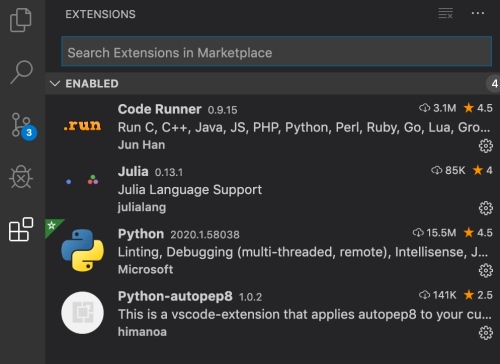
我非常喜歡用另一個免費(開源?) IDE, VS Code (Visual Studio Code) for python script coding and debugging. VS Code 是 Microsoft 提供的免費軟體。不但是跨Windows/MacOS/Linux 平台,同時支持多種 programming language, 包含 Python, Javascript, Julia, etc. VS Code 有許多外部插件, 可以擴充 VS Code 的功能,包含多種 programming language 的支持。下圖就是和 python/julia 相關的基本插件:Python (linting, debugging), Code Runner (run code), Autopep8 (formatter).

另外 VS Code native 整合 git (revision control and remote repository), 支持 virtual environments: virtualenv and conda. 對於測試不同 python versions 和 packages 很方便。
VS Code 非常適合 debug 輕量級 scripting and fast prototyping.
最常見的 debugging 方法就是 print(variable). 主要的優點是不需要額外的工具或設定。 兩個缺點:(1) 切換 debugging (enable printing) and non-debugging (disable printing) 很麻煩。 (2) Print 比較難定位 function and context, 特別有多個 python files.
除了 IDE debugging 和 print debugging 兩個極端,是否有介於之間的 debugging 方法? 答案是肯定的。這裏介紹兩種工具:PySnooper and Logging.
PySnooper 號稱是 Poor man's python debugger. [@rachumPySnooper2020], [@jackPythonDiaoShiShenQiZhiPySnooper2019], [@cvPythonGaoBiePrint2019] Github 開源的 PySnooper,允許和print執行相同的操作,只需向感興趣的函數添加一個裝飾器行,而不是小心地創建正確的列印行。將會得到函數的詳細日誌,包括運行了哪些行、何時運行、以及何時更改了局部變量。
很多參考文章,此處不贅述。
[@unknownPythonLogging2012] and [@leiReplaceYour2014]
Direct input
Use dict: Method 1: 一筆一筆加入。
import pandas as pd
dict1 = {'Name': 'Allen' , 'Sex': 'male', 'Age': 33}
dict2 = {'Name': 'Alice' , 'Sex': 'female', 'Age': 22}
dict3 = {'Name': 'Bob' , 'Sex': 'male', 'Age': 11}
data = [dict1, dict2, dict3]
df = pd.DataFrame(data)

>>> df
   Age   Name     Sex
0   33  Allen    male
1   22  Alice  female
2   11    Bob    male
Method 2: 一次加入所有資料。
import pandas as pd
name = ['Allen', 'Alice', 'Bob']
sex = ['male', 'female', 'male']
age = [33, 22, 11]
all_dict = {
    "Name": name,
    "Sex": sex,
    "Age": age
}
df = pd.DataFrame(all_dict)

>>> df
    Name     Sex  Age
0  Allen    male   33
1  Alice  female   22
2    Bob    male   11
import pandas as pd
df = pd.read_csv('xxx.csv')
>>> df.head(2)
   Age   Name     Sex
0   33  Allen    male
1   22  Alice  female
>>> df.tail(2)
   Age   Name     Sex
1   22  Alice  female
2   11    Bob    male
>>> df.shape
(3, 3)
>>> df.info()
<class 'pandas.core.frame.DataFrame'>
RangeIndex: 3 entries, 0 to 2
Data columns (total 3 columns):
Age     3 non-null int64
Name    3 non-null object
Sex     3 non-null object
dtypes: int64(1), object(2)
memory usage: 152.0+ bytes
>>> df[0:2]
   Age   Name     Sex
0   33  Allen    male
1   22  Alice  female
>>> df['Name'][0:2]
0    Allen
1    Alice
Name: Name, dtype: object
>>> df[['Name','Age']][0:2]
    Name  Age
0  Allen   33
1  Alice   22
>>> df.count()
Age     3
Name    3
Sex     3
dtype: int64
>>> df[df['Layer'] == 'Conv2d'].count()
可以參考 [@ithomeDi142016]
# select rows by conditions
dfPlot = df[df['Layer']=='Conv2d']
dfPlot.reset_index(inplace = True)

# select columns by name
dfPlot = dfPlot[['Layer', 'ChI', 'ChO']
Python plot 使用標準 matplotlib.pyplot.
import matplotlib.pyplot as plt

def dfPlot(df):

    dfPlot = df[df['Layer'] == 'Conv2d']
    dfPlot = dfPlot[['Layer', 'ChI', 'IFmapX', 'IFmapY', 'ChO', 'OFmapX',
                     'OFmapY', 'ParamW', 'MAC', 'MAC2W', 'MAC2IF', 'MAC2OF']]
    dfPlot.reset_index(inplace=True, drop=True)

    logger.debug("dfPlot size = \n%s" % (dfPlot.count()))
    logger.debug("dfPlot = \n%s" % (dfPlot))

    plt.style.use("ggplot")
    plt.figure()
    #plt.plot(dfPlot.index, dfPlot['ParamW'])
    plt.plot(dfPlot.index, dfPlot['MAC2W'])
    plt.plot(dfPlot.index, dfPlot['MAC2IF'])
    plt.plot(dfPlot.index, dfPlot['MAC2OF'])
    plt.xlabel('layer')
    plt.ylabel('loss')
    plt.show()
更方便是直接用 pandas.DataFrame.plot function. 實際的例子如下。要加上 plt.show() 出圖。使用 Jupyter notebook 可以忽略 plt.show().
import tensorflow
import keras
import pandas as pd
import numpy as np
import math
import random
import matplotlib.pyplot as plt
# #Generate a sin wave with no noise
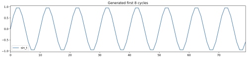
# First, I create a function that generates sin wave with/without noise. Using this function, I will generate a sin wave with no noise. As this sin wave is completely deterministic, I should be able to create a model that can do prefect prediction the next value of sin wave given the previous values of sin waves!
#
# Here I generate period-10 sin wave, repeating itself 500 times, and plot the first few cycles.
def noisy_sin(steps_per_cycle = 50,
number_of_cycles = 500,
random_factor = 0.4):
'''
random_factor : amont of noise in sign wave. 0 = no noise
number_of_cycles : The number of steps required for one cycle
Return :
pd.DataFrame() with column sin_t containing the generated sin wave
'''
random.seed(0)
df = pd.DataFrame(np.arange(steps_per_cycle * number_of_cycles + 1), columns=["t"])
df["sin_t"] = df.t.apply(lambda x: math.sin(x * (2 * math.pi / steps_per_cycle)+ random.uniform(-1.0, +1.0) * random_factor))
df["sin_t_clean"] = df.t.apply(lambda x: math.sin(x * (2 * math.pi / steps_per_cycle)))
print("create period-{} sin wave with {} cycles".format(steps_per_cycle,number_of_cycles))
print("In total, the sin wave time series length is {}".format(steps_per_cycle*number_of_cycles+1))
return(df)
steps_per_cycle = 10
df = noisy_sin(steps_per_cycle=steps_per_cycle,
random_factor = 0)
n_plot = 8
df[["sin_t"]].head(steps_per_cycle * n_plot).plot(
title="Generated first {} cycles".format(n_plot),
figsize=(15,3))
plt.show()

iThome, Tony. 2016. “[第 14 天] 常用屬性或方法(3)Data Frame.” iT
邦幫忙::一起幫忙解決難題,拯救 IT 人的一天. 2016.
https://ithelp.ithome.com.tw/articles/10185922.
TBA
Reference
iCoding – We Coding …: http://icodingtw.blogspot.com/2012/08/logging.html
[Python] logging 教學: https://stackoverflow.max-everyday.com/2017/10/python-logging/
替换你的print(logging模块超简明指南): https://www.zlovezl.cn/articles/replacing-print-simple-introduction-to-logging/
Debug method in Python
1. IDE:
VS Code, PyCharm
2. Command line base
Poor man’s debugging tool: peeping variable
Logging package
垂直和平行都是幾何最重要的基石。
歐幾里得平面幾何五大公理。最後一個公理就是平行公理:一條直線線外一點只能做出唯一平行直線。
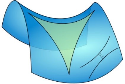
俄國數學家羅巴切夫斯基 (Lobachevsky) 一輩子想要其他公理證明平行公理或者用更直觀的公理取代平行公理都未能成功。後來用反證法:一條直線外一點一定會有兩條或兩條以上的平行直線,試圖找出矛盾。但卻發現邏輯自洽。因而開創非歐幾何學。我們現在知道這其實對應雙曲面幾何如下。這是一個馬鞍面,立起來就是一個雙曲面。雙曲面上的"直線“線外一點可以找到無數 diverged “直線”,和原來的“直線”永不相交,因此可以有無數條平行線。
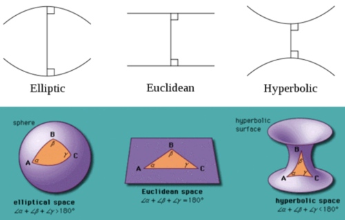
黎曼則另闢蹊徑開拓黎曼幾何學。對應(橢圓)球面幾何。球面上所有的“直線”都是 中心在球心的封閉大圓。因此所有的“直線”都相交。平行公理變成一條直線外一點沒有任何平行直線。常見的誤區是球面的緯線是平行線。緯線除了赤道是“直線”,其他的緯線都是球面上的“曲線”,不能視為平行直線!
下圖很好的總結三種幾何學。
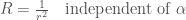
曲面幾何可以定義曲率。曲率乍看之下是把一個曲面放在更高維空間(外)顯出的性質。
例如上圖是把二維的曲面放在(嵌入)三維的歐氏空間,可以明顯看出不同的曲面。同時可以定量的描述這個曲面的曲率。例如球面的曲率非常直觀和球的半徑相反。越小的球,曲率越大。但球面曲率是一個整體的性質,還是每一點(和其鄰近點)的性質?曲率是和半徑成反比,還是和半徑平方成反比?
先回顧二維歐氏平面上的一維曲線。很明顯曲線上每一點(和其鄰近點)都可以定義“線曲率” 

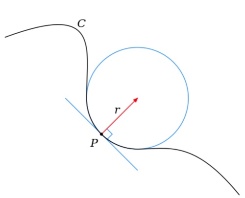
再回到二維曲面,曲面上每一點都有無限條曲面上的曲線相交於這一點。每一條曲線都有本身的“線曲率”,可以是正或負。高斯曲率定義二維曲面每一點的“曲面曲率” 


以完美球面為例,每一點所有相交曲線的線曲率都一樣。都是大圓(圓心即是球心)半徑的倒數。所以球面每一點的高斯曲率 
如果是非完美球面,例如橢圓球面半徑為 

再考慮雙曲面幾何。每一點相交曲線的”線曲率“必定有正有負,
So far so good!
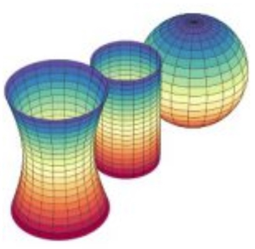
檢查高斯曲率在平面和圓柱面的曲率。平面是 trivial case, 所有 


顯然這不直觀。直觀上會認為圓柱面和平面不同,具有曲率,至少在 x,y 方向有曲率。為什麼高斯會定義高斯曲率為 

圓柱面是一個很好的例子,說明外顯曲率和內稟曲率的不同。
是嵌入在二維或是更高維歐氏空間,所以“線曲率”是外顯曲率。 或是 mean curvature =
  應該也是外顯曲率。NO!, 結果剛好等於最大和最小線曲率的乘積 . 高斯自己似乎也覺得不可思議,稱為"絕妙定理“[@wikiTheoremaEgregium2019] 如下。
除了平行公理可以用來分類不同的曲面,是否有其他更直觀的特徵分類?
Yes! 可以用三角形內角和是否大於,等於,或小於 
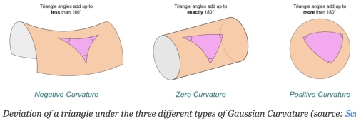
另外一個特徵是圓周率。在平面幾何任意圓的周長除以直徑永遠等於
但在曲面則會小於或大於
以上特徵(三角形內角和,圓周率)不只是定性的描述,都和高斯曲率有定量的關係。更重要的是這是曲面內稟的特性!就是在曲面的生物,就可以測量到高斯曲率。
下表總結三種幾何學:
| Geometry | Sphere 球面 | Plane 平面/柱面 | Hyperbolic 雙曲面 |
|---|---|---|---|
| Creator | Riemann | Euclid | Lobachevsky |
| 平行公理平行線 | 0 | 1 |  |
| 三角內角和 |  |
|
 |
| 圓周率 | |
|
|
| 高斯曲率 |  |
 |
 |
上表的平行線,三角內角和,圓周率都是 global (全域) 特性。但是高斯曲率卻是 local (局部) 特性。如何連結 global and local?
圓周率 Bertrand–Diguet–Puiseux theorem (Wifi 2019a). 是否有積分形式?
三角形內角和 (Gauss-Bonnet theorem (Wiki 2019a)
A good article to integrate everything including Laplacian using unit volume (Gray and Vanhecke 1979).
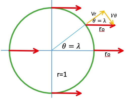
一個明顯的問題是平行公理是 global 的特性(直線永不相交),是否有直接對應局部曲率的公式? Yes,平行移動 parallel transport 就是平行的微分定義!! 和曲面微分幾何有非常深層的連結。
反向問題:既然可以用三角內角和以及圓周率極限定義曲率,還需要用平行定義取率嗎? Absolutely Yes, 平行觀念和座標 grid line and local basis vector 定義吻合(local basis vector = grid line 的切線),可以直接融入純量場,向量場,張量場的微分運算。 相反三角內角和或圓周率基於極限的定義在各種微分幾何的運算並不實際。
(Keng 2018) 剛好和我想的一致,平行公理和 parallel transport.
(Wiki 2019a) 微分幾何對平行移動的定義:
平行移動是將流形上的幾何特性沿著光滑曲線移動的一種方法。如果流形上有一個 affine connnection(covariant derivative),那麼 affine connection 保證我們可以將流形上的向量沿著曲線移動使得它們關於這個 connection 保持「平行」。
在某種意義上說,關於 connection 的平行移動提供了將流形的局部幾何沿著曲線移動的方法:即「連接」了鄰近點的幾何。有許多種平行移動的概念,但其中一種方式等同於提供了一個 connection。事實上,通常的 connection 是平行移動的無窮小類比。反之,平行移動是 connection 的局部實現。
因為平行移動給出了 connection 的一種局部實現,它也提供了曲率的一種局部實現(holonomy)。Ambrose-Singer 定理明確了曲率與 holonomy 的關係。
簡言之,平行移動基本是一種 local connection, 以及實現 curvature 的方式。
問題是:平行移動和平行公理有什麼關係?
平行公理:一條直線和線外一點平行直線的關係。
什麼是直線?最直觀的定義就是最短路徑,在非平面的“直線”看起來並不直。
數學的表示是: 
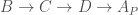
平面幾何:平行移動先定義 Geodesic A, 接著線外一點 P, 可以找到一條 Geodesic B 垂直於 A at T. 再來根據平行公理,只有一條平行線 Geodesic C 平行於 A, 且垂直於 B. 因為 A 和 C 是平行線,永不相交。為了讓 parallel transport 形成封閉迴路 (holonomy), 可以在 A 上找一點 Q, 並且做垂直線到 C, 稱為 geodesic D.
此時從 

柱面幾何:直接剖面切開就是平面。parallel transport 和平面一樣。如果沿著三角形 holonomy, 因為內角和為 180, 回到起點的 parallel transport 夾角為 0. Gauss curvature 為 0.
錐面幾何:圓錐面如下圖(a)的曲率?圓錐面可以展開成平面缺角圓形如下圖(b). 除了 A 點之外任何點的曲率為 0. 因為錐面上一個 close loop, 如果不包含 A, parallel transport 夾角為 0. 因此曲率為 0.
如果包含 A 的圓,parallel transport 夾角 = 


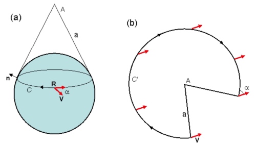
另一個問題,上圖球面非大圓 R 的 parallel transport 夾角? 常見的回答是 0. 錯誤的答案!正確的答案是用圓錐面和球面的切線為 R,再展開如上圖 b.
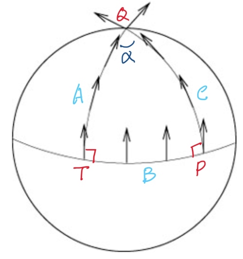
球面幾何:平行移動先定義 geodesic A (上圖左邊弧線), 赤道的 geodesic B 垂直於 A at T. 由平行定理我們知道球面幾何不存在和 A 平行(不相交)的 geodesic. 我們只能選擇和 B 垂直的 geodesic C, given we know A 和 C 會相交於 Q 點(其實在北極)。
此時從 


如果只是在局部做一個封閉迴路(holonomy),局部看起來就像歐氏空間。Parallel transport 的 holonomy 夾角為 0. Use Gauss curvature
雙曲線幾何:直接考慮鞍面的三角形,內角和小於 180. parallel transport 為負夾角。
Parallel Transport 


Parallel transport 更數學而且和座標系無關的定義:
一個類比:如果不是一個向量 

平行移動和等高線的數學公式雖然非常類似。問題的形式 (formulation) 卻不同。
平行移動是給定一條任意線 

等高線是給定一個純量場
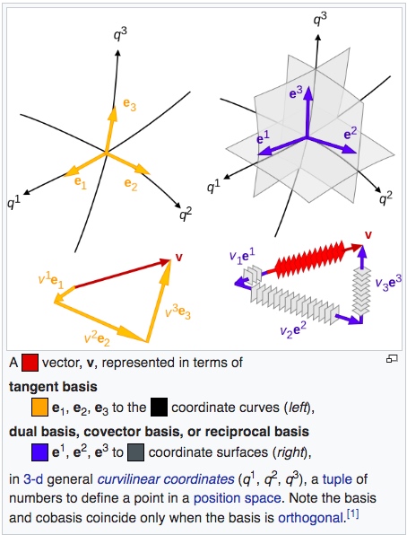
張量(tensor) 最重要的特性就是座標系無關,可用於平面或曲面。張量分為三類:
 , basis vector scale up, dual basis vector scale down, 張量分量也會 scale up. 其他特性和一般張量一樣。
其他的張量運算下面展開。
在卡氏座標系(笛卡爾直角座標系):
曲線和切向量:
注意:千萬不要用 ![[u_1, u_2]](https://s0.wp.com/latex.php?latex=%5Bu_1%2C+u_2%5D+&bg=fff&fg=444444&s=0&c=20201002)
先考慮 gradient operator,
一個純量場(0階張量)的梯度, 
一個一維量場的梯度, 
純量場的方向導數,基本上是純量場的梯度 (gradient) 和方向向量的內積。
(1) 只能用於卡氏座標系。接下來幾個重點:1.座標系無關;2.推廣到曲面;3.簡化公式。
現在引入 covariant/contravariant basis and tensor, 和愛因斯坦 summation notation.
Basis vectors
Dual basis vectors 
注意 


對於歐氏空間非直角座標系,(1) 可以修改為:
使用愛因斯坦 notation 重寫 (4)
曲面空間的純量場方向導數和 (5) 完全相同。因為純量場是 basis invariant.
但是曲面空間的向量場是 basis covariant or contravariant, 所以曲面的向量場的方向導數會比歐氏空間複雜的多。
曲面空間向量場
$latex \vec{V} = V^1 \mathbf{e_1} + V^2 \mathbf{e_2}
= V^{\alpha} \mathbf{e_\alpha} \\
\vec{u} = u^1 \mathbf{e_1} + u^2 \mathbf{e_2} $
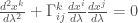
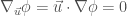
$latex \nabla_{\vec{u}}\vec{V} = \vec{u}\cdot\nabla\vec{V}
= (u^1 \mathbf{e_1} + u^2 \mathbf{e_2})\cdot\nabla\vec{V} \\
\nabla_{e_\beta}\vec{V}=\mathbf{e_\beta} \cdot\nabla\vec{V}
= \mathbf{e_\beta} \cdot\nabla (V^\alpha \mathbf{e_\alpha})
= \mathbf{e_\beta} \cdot \frac{\partial(V^\alpha \mathbf{e_\alpha})}{\partial e_i} \mathbf{e^i} \\
= \frac{\partial(V^\alpha \mathbf{e_\alpha})}{\partial e_\beta}
= \frac{\partial V^\alpha}{\partial e_\beta}\mathbf{e_\alpha} +
V^\alpha \frac{\partial \mathbf{e_\alpha}}{\partial e_\beta}
= \frac{\partial V^\alpha}{\partial e_\beta}\mathbf{e_\alpha} +
V^\alpha \Gamma^k_{\alpha\beta}\mathbf{e_k} \\
= \frac{\partial V^\alpha}{\partial e_\beta}\mathbf{e_\alpha} +
V^i \Gamma^{\alpha}_{i\beta}\mathbf{e_\alpha}
= (\frac{\partial V^\alpha}{\partial e_\beta} +
V^i \Gamma^{\alpha}_{i\beta})\mathbf{e_\alpha} $
此處利用 Christopher symbol 以及
$latex \frac{\partial \mathbf{e_\alpha}}{\partial e_\beta} =
\Gamma^k_{\alpha\beta}\mathbf{e_k} $
如果是歐氏空間且直角座標系,Christopher symbol
如果是歐氏空間但極座標系,因為每一點的 local basis vector 方向都不同,Christopher symbol 不為 0, 一共有 2x2x2=8 個 components [@cyrilChristoffelSymbol2016].
愛因斯坦 notation and convention: 向量場的梯度微分是二階張量(樓上加樓下)。

最後 $latex \nabla_{\vec{u}}\vec{V} = \vec{u}\cdot\nabla\vec{V}
= (u^1 \mathbf{e_1} + u^2 \mathbf{e_2})\cdot\nabla\vec{V}\\
= u^\beta (\frac{\partial V^\alpha}{\partial e_\beta} +
V^i \Gamma^{\alpha}_{i\beta})\mathbf{e_\alpha}
= (u^i \frac{\partial V^k}{\partial e_i} +
u^i V^j \Gamma^{k}_{ij})\mathbf{e_k}
= (u^i {\partial_i V^k} +
u^i V^j \Gamma^{k}_{ij})\mathbf{e_k} $
愛因斯坦 notation and convention: 向量場的方向導數是一階張量(樓上)。
 , 只有一個樓上 index,代表一階張量 contra-variant.
  , 只有一個樓下 index,代表一階張量 co-variant (one-form).
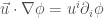 , 張量和 1-form 張量內積結合,同一個 index i 樓上樓下抵銷,變成 0 階張量(純量)。(0 階張量)得到一階 one form 張量;(一階張量)得到二階張量;以此類推。
 是二階(樓上加樓下)tensor.
 是一階(樓上) 張量。
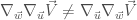 . 事實上,
 ? (TBC)
曲線和切向量回顧:
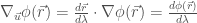
純量場的線方向導數
其實這就是著名的 gradient theorem, 或是線積分基本定理推廣到曲面。重點是曲面線積分是路徑無關!或是封閉迴路線積分為 0. 但在向量場不是如此。
$latex \int_p^q \nabla_{\vec{u}}\phi(\vec{r}) d\lambda
= \int_p^q \nabla\phi(\vec{r})\cdot d\vec{r} = \phi(q) – \phi(p) $
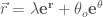
Let 
射線運動卡氏座標系:


射線運動極座標系:

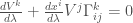
向量場的線方向導數,稱為絕對導數(absolute derivative)
$latex \nabla_{\vec{u}}\vec{V}(\vec{r}) = \frac{d\vec{r}}{d\lambda}\cdot\nabla\vec{V}(\vec{r}) \\
= u^i {\partial_i V^k} + u^i V^j \Gamma^{k}_{ij}
= \frac{d V^k}{d\lambda} + \frac{d x^i}{d\lambda} V^j \Gamma^{k}_{ij} $


積分形式: 


另一個重點是 

卡氏座標系:

極座標系:

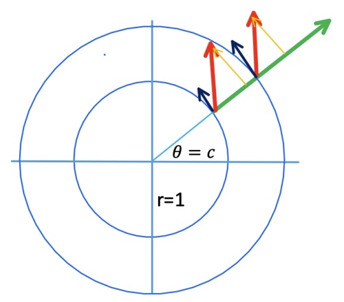
Example 1: 射線運動 (起點在r=1上)
Let 
Example 2: 圓周運動
Let 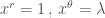


Gray, A., and L. Vanhecke. 1979. “Riemannian Geometry as Determined by
the Volumes of Small Geodesic Balls.” Acta Mathematica 142: 157–98.
https://doi.org/10.1007/BF02395060.
Keng, Brian. 2018. “Hyperbolic Geometry and Poincaré Embeddings.”
Bounded Rationality. June 17, 2018.
http://bjlkeng.github.io/posts/hyperbolic-geometry-and-poincare-embeddings/.
Wiki. 2019a. “Gaussian Curvature.” Wikipedia.
https://en.wikipedia.org/w/index.php?title=Gaussian_curvature&oldid=910677726.
———. 2019b. “Parallel Transport.” Wikipedia.
https://en.wikipedia.org/w/index.php?title=Parallel_transport&oldid=911069387.
———. 2019c. “Theorema Egregium.” Wikipedia.
https://en.wikipedia.org/w/index.php?title=Theorema_Egregium&oldid=895212511.
黎曼微分幾何是廣義相對論的數學基礎。張量分析是黎曼微分幾何的必備數學工具。
由於相對論的影響,不同(運動)觀察者所量測的物理定律 (e.g. least action principle) 都要一樣。這剛好對應幾何不同座標系的“不變性”。不變的 scalar 可以使用 invariant. 不變的 vector/tensor, 因為分量仍然和座標系相關,我們用 covariant 表述。
不同(運動)觀察者對應幾何不同座標系. 不要執著一個是動態,一個是靜態。這裏所說的幾何座標系都包含時間軸 (
一條 wordline 是相對於一個觀察者(座標系)。例如 A 觀察到一個靜止物體 S,在 A 的(直角)座標系 S 的位置就是一條垂直的 world line. B 是一個相對 A 定速 
有兩個方法:
(i) B 創造自己的(直角)座標系以及 S 的 world line. 顯然在 B 的直角座標系 S world line 是一條斜線。斜率是 

我們關心 S 的運動 (object oriented) 一次看到 A 和 B 座標系的詮釋,見 (ii). 這對廣義相對論研究時空內稟幾何特性很重要。
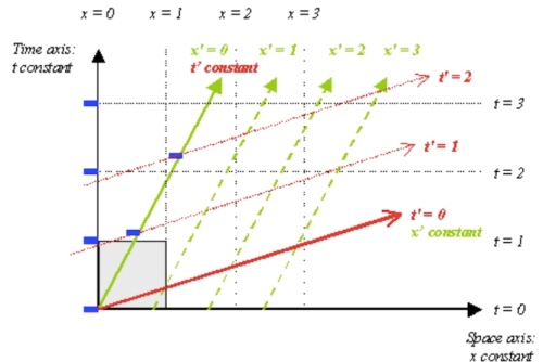
(ii) 在 A 的直角座標系 (grid line) 重劃 B 的(非直角)座標系 (grid line)。同一條垂直的 world line, 在 A 座標系 grid line 是靜止;但在 B 座標系 grid line 則是運動。
下圖是一個例子。A 觀察者是直角座標系 


注意這種重劃座標系網格並不限於相對速度固定的觀察者。原則上適用任何運動觀察者。假設觀察者 C 是相對于 A 有固定等加速度。也可以定義 


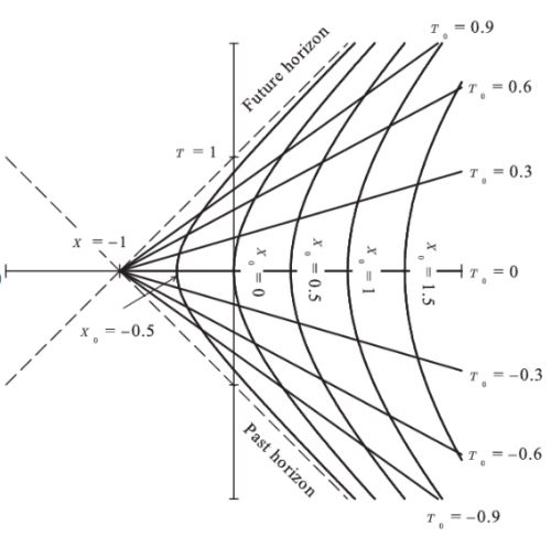
 幾何的一條世界線 C (不是面或其他形狀) 幾何的不同座標系以及網格
物理定律
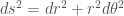
微分幾何的 1st fundmental form 

注意微分幾何的 1st fundamental form 可以推廣到 curved space or coordinate. 這裏使用愛因斯坦 summation notation.
牛頓第二定律: 

最小作用力原理 (Least action principle) 是比牛頓運動定律更基本的定理。分析力學首先找到 Lagrangian 


舉一個例子:古典力學 Lagrangian of free particle (no potential field) in Cartesian and polar coordinate. [@ActionPhysics2019]
$latex L =\frac{1}{2} m v^2=\frac{1}{2} m (\dot{x}^2 + \dot{y}^2)
\quad L =\frac{1}{2} m (\dot{r}^2 + r^2 \dot{\varphi}^2) $
最小作用原理推廣到 4D 時空 for two events 


但在相對論力學 4D 時空的 Lagrangian of free particle (no potential field). [@RelativisticLagrangian2019] 


UTM. 2018. “Proper Time, Coordinate Systems, Lorentz Transformations | Internet Encyclopedia of Philosophy.” 2018. https://www.iep.utm.edu/proper-t/.
Coordinate invariant 基本是 scalar quantity or field, 例如
Contravariance 基本是 vector/tensor, 例如 curvature tensor, …. 什麼是 contravariant? 


Covariance 也是 vector/tensor, 為什麼是 covariance? 一個例子是 gradient of scalar field. 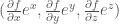

歐式空間(或是 tangent space on manifold)
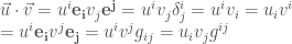
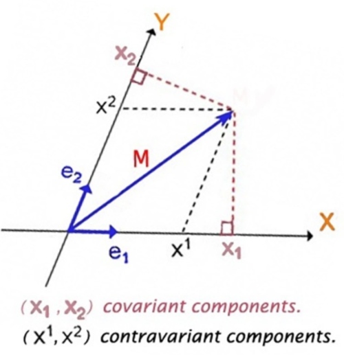
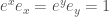
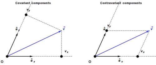
如何在座標系表達一個向量 
選擇一組 basis vectors (假設不正交). 然後分解成 basis vectors 的平行分量 (下圖右 typo 

我們稱 


問題是如何用數學式計算
如果是在直角座標系如下,可以看出 contra-variant!

顯然在非直角座標系是錯的!正確的數學表述在後面。
此時稱
下一個問題,是否還有其他方法表示一個向量?Yes!
我們可以用垂直投影分量表示一個向量 (下圖左, 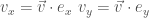
我們稱 


問題是如何找到對應的 (cotangent) basis vector 
為了滿足 


也就是說 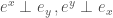
注意 

此時可以用新的 (cotangent) basis vector 表示:
因為 


Inner Product Using Einstein Notation
Scalar field is invariant.
Vector/tensor field is contravariant.
Gradient of scalar field is a vector field, which is co-variant.
為了直觀了解 curved coordinate and space, 用以下的順序理解:直角座標系
orthonormal 座標系
scaled 座標系
Non-orthogonal 座標系
Polar 座標系
三維空間
推廣上述二維的垂直觀念到三維空間。


同理 
推廣到 n 維空間:
Tangent basis: e1, e2, …, en, C(n,1)=n
Reciprocal basis: e1.,… C(n, n-1) = n
Curved Space or Coordinate System
Basis Vector
Reciprocal Basis Vector


Covariant derivative 是 directional derivative 的推廣。同樣用以下的順序理解:直角座標系
Scalar field: 
Scalar field:
Scalar field: 


$latex \nabla f(r,\theta) = \frac{\partial f}{\partial r} e^r + \frac{\partial f}{\partial \theta} e^\theta \quad\text{(1- form, covariant)}\\
= \frac{\partial f}{\partial r} e_r + \frac{1}{r^2}\frac{\partial f}{\partial \theta} e_\theta \qquad\text{(contra-variant)} $
另外常見的表示法是 Euclidean metric, normalized form, 
一個純量場(0階張量)的梯度,
一個一維量場的梯度,
 , 最小作用原理~?。 Geodesic.
Wiki. 2019. “Covariance and Contravariance of Vectors.” In Wikipedia.
https://en.wikipedia.org/w/index.php?title=Covariance\_and\_contravariance\_of\_vectors&oldid=904269873
“Action (Physics).” 2019. Wikipedia.
https://en.wikipedia.org/w/index.php?title=Action_(physics)&oldid=904671703
Cyril. 2018. “Geodesic Equation from the Principle of Least Action.” September 18, 2018.
http://einsteinrelativelyeasy.com/index.php/general-relativity/97-geodesic-equation-from-the-principle-of-least-action.
“Relativistic Lagrangian Mechanics.” 2019. Wikipedia.
https://en.wikipedia.org/w/index.php?title=Relativistic_Lagrangian_mechanics&oldid=884947845
Example 1: 牛頓空間以及不同慣性運動觀察者


 座標系。為了簡化在 2D plan,只考慮. 垂直軸是 軸。
Example 2: 狹義相對論慣性運動觀察者
Example 2: 廣義相對論