allenlu2007

A great WordPress.com site

Month: April, 2014

HMM 幾個有趣應用

by allenlu2007

Hidden Markov Model (HMM) 的理論基礎清晰,有許多有趣的應用。本文 highlight 幾個常見的應用。

這些應用也常用 neural network 來處理。比較起來,neural network 的理論似乎比較 fuzzy. 


Application 1:  Optical Character Recognition (OCR)

可以參考本文為 tutorial.  

幾個重點

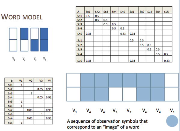
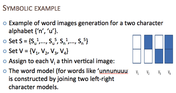
1. 字母的 image 是來自 sequences of thin vertical images (segments), 示意如下:

NewImage

1a. Feature extraction: image 本身是 (i) high dimensional; (ii) distribution instead of discrete values

所以需要 (i) feature extraction to reduce dimension; and (ii) clustering by K-mean or GMM and then discretisation (quantisation)

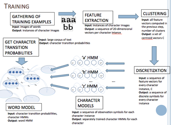
2. 每一個字毋 (a, b, c, .., z) 都有自己的 character HMM (26 個 character HMM not counting 大小寫)

3. Merge character HMM into word HMM. 整個就是一個大的 HMM.  

4. 一開始先用 character training 自己的 HMM (Baum-Welch EM algorithm).  

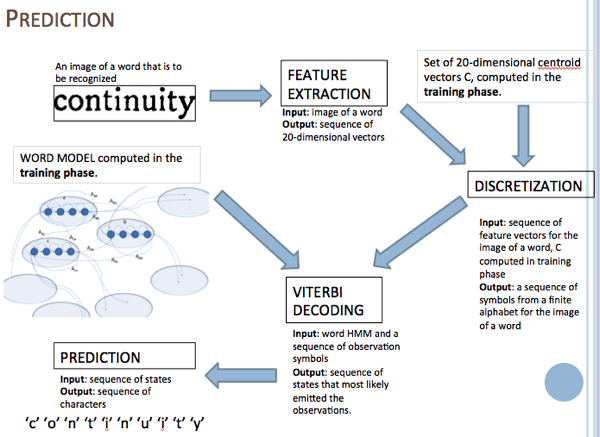
5. Given a new image of word, use the word HMM to predict the most likely sequence of characters. 如何 train word? 或是不用 train.?

6. Use EM to determine the transition probability matrix and emission probability matrix.    Use Viterbi algorithm to determines the most likely character and word.

NewImage 


兩個 phases:

NewImage


and 

NewImage


Q&A

How to do word model training???  It is only one HMM.


Application 2:  Speech Recognition

可以參考本文

 基本的 idea 和 OCR 類似:

1. Feature extraction

2. Assign feature extraction vector (high dimensional) to HMM states

3. Baum-Welch forward-backward training assigns transition and emission probabilities from each HMM state

4. Viterbi training assigns feature vector to a particular state


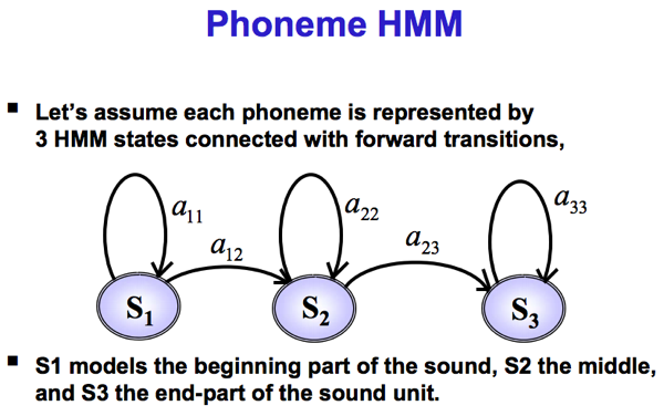
類似 OCR 中的 character, speech recognition 的基本單位是 phoneme.  每一個 phoneme 都有自己的 HMM.

NewImage


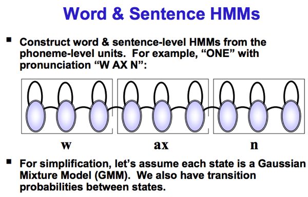
Word and sentence level HMMs from phoneme-level unit 如下

NewImage


Application 3:  Gesture Recognition

可以參閱本文


以上的應用都有

(1) image or voice input into segment

(2) feature extraction (may be high dimensional)

(3) clustering and discretisation (quantisation) to finite output values

(4) build HMM and use Baum-Welch EM algorithm to train transition and emission probability

(5) Input real data and use Viterbi to find the best sequence


Q&A

如何中英文混合 speech recognition or 英文 speech recognition for Chinese?


Application 4:  Biology – Gene Prediction, Protein Unfold


Baum-Welch (EM) Algorithm for HMM

by allenlu2007

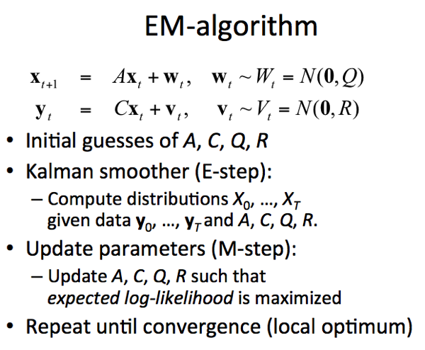
前文提到 EM algorithm for Kalman filter training.

Step 0:  Initial guess 

A, C, Q, R, pi (initial mean), v (initial covariance)

Step 1: Kalman filter forward pass

Step 2: Kalman smoothing (Rauch) backward pass

Step 3: Update A, C, Q, R to maximize the Q function!  

Step 4: Repeat step1 till converge.


Key is step 3:  先 compute joint pdf p(x1, .. , xn, y1, …, yn)

Q function derivative in terms of joint pdf!


在 HMM 中,有類似的 EM algorithm, 即是 Baum-Welch algorithm.  但更簡化

(1) A and Q becomes matrix A (transition probability matrix)

(2) C and R becomes matrix B (emission probability matrix)

(3) Initial probability theta vector


其實就是把 Gaussian pdf (mean and covariance) 換成 probability matrix/vector!!!!!!


Step 0: Initial guess of A, B, pi

Step 1: Forward pass using HMM filtering

Step 2: Backward pass using HMM smoothing

NewImage


Step 3: EM algorithm to maximize Q function

Step 4: repeat step 1 and check converge


Details:

Step 0: Initial guess of A, B, pi

A: NxN  (N states)

NewImage

B: KxN  (K possible output values)

NewImage

Pi:  Nx1 vector

NewImage

NewImage

Step 1: Forward pass using HMM filtering

NewImage

Step 2: Backward pass using HMM smoothing

NewImage

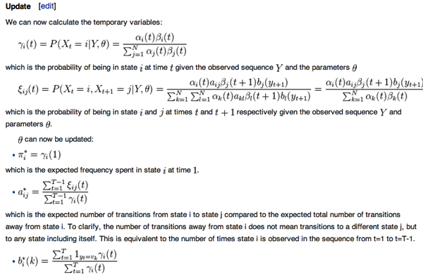
Step 3: Update using EM algorithm to maximize Q function

NewImage

詳細推導過程見最後。


Step 4: repeat step 1 and check converge

It is possible to over-fit a particular data set. That is P(Y|\theta_{final})>P(Y|\theta_{true}). The algorithm also does notguarantee a global maximum.


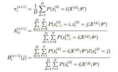
Baum-Welch Algorithm 推導

Z is state {1..M}, the latent variables;  X is observations {1.. N}

NewImage

NewImage

Baum-Welch is an EM algorithm

NewImage

Q-function

NewImage 

NewImage 

Then use the Lagrange multiplier to find the maximum

NewImage


NewImage

HMM vs. Kalman Filter 異同; Baum-Welch, Viterbi, EM algorithm 異同

by allenlu2007

Kalman filter and smoother 和 HMM filter 的異同

HMM or Baysian filter:

1. discrete state

2. probabilistic model

3. transition probability and emission probability matrix

4. PMF; no assumption of Gaussian or linear what so ever 


KF is a special case of HMM

1. continuous state (and infinite states)!

2. state space model 

2. linear state space model!! Very strong assumption!

3. Transition pdf and emission pdf are all Gaussian.  Therefore, everything is Gaussian


State, transition, and emission pdf are Gaussian PDF

Therefore, the estimate state = mean of the PDF, and covariance matrix of the PDF

細節可以參考 Hidden Markov Model of Filtering, Smoothing.


Kalman filter and smoother 和 HMM Viterbi algorithm 的不同

Viterbi 是假設 transition and emission probabilities 為已知,根據觀察到的 data 決定最有可能的 state sequence, i.e. P(x1, x2, .., xk | y1, y2, … yk)

Kalman filter/smoother 是假設 transition and emission pdf (Gaussian) 為已知,根據觀察到的 data 決定最有可能 state conditional probability  P(xk | y1, y2, .. yk or yn) at k-th moment (point-wise)!  yk is Kalman filter, yn is Kalman smoother.

HMM 是否可以有 point-wise 的 estimation like Kalman filter.  答案是 yes.  但是 HMM with finite state 和 linear space 一個很不同的特性是有些 transition 是禁止的 (probability = 0,想想 convolution code or trellis code modulation).  如果只做 point-wise estimation, 最後可能得到錯誤的 transition (就 overall sequence probability = 0)!  可以參考本文 for more information of Viterbi algorithm.


Kalman filter and Convolution Code and HMM 比較

Kalman filter: linear space model ->  state is continuous Gaussian PDF -> observed data is continuous Gaussian PDF

HMM: state is discrete (finite or infinite) -> transition probability matrix and emission probability matrix

Convolution code or Trellis code: state is finite discrete -> transition probability matrix is known. observed data is  continuous Gaussian PDF

Therefore, Kalman filter is applied to linear space model, ML on the point-wise of given data (Kalman filter/smoother)

HMM and Convolution code/Trellis code decode with known transition probability and emission probability matrix/Gaussian PDF,  ML on the sequence of given data using Viterbi algorithm.

The Convolution code/Trellis code decoding has two flavors: one is called hard decision, quantized the received data to the finite output states like HMM.   Or soft decision, no quantization.   The soft decision performance is better than hard decision because it keeps more information.


Kalman filter EM algorithm 和 HMM Baum-Welch algorithm 異同

Baum-Welch algorithm 是用在 HMM, 基本上和 EM algorithm used for Kalman filter 是類似的 algorithm.

Baum-Welch algorithm in HMM 相當於 EM algorithm in Kalman filter.  Unknowns 有些不同,forward and backward pass 相同。


HMM Baum-Welch algorithm 和 HMM Viterbi algorithm 的不同

簡單來說,Viterbi algorithm 是假設 transition and emission probabilities 為已知,根據觀察到的 data 決定最有可能 的 state sequence.  

Baum-Welch algorithm 則是 transition and emission probabilities 為未知,根擄觀察的 data 決定最有可能的 transition, emission probability, and initial state probability distribution.

The Baum-Welch algorithm and the Viterbi algorithm calculate different things.

If you know the transition probabilities for the hidden part of your model, and the emission probabilities for the visible outputs of your model, then the Viterbi algorithm gives you the most likely complete sequence of hidden states conditional on both your outputs and your model specification.

The Baum-Welch algorithm gives you both the mostl likely hidden transition probabilities as well as the most likely set of emission probabilities given only the observed states of the model (and, usually, an upper bound on the number of hidden states). You also get the “pointwise” highest likelihood points in the hidden states, which is often slightly different from the single hidden sequence that is overall most likely.

If you know your model and just want the latent states, then there is no reason to use the Baum-Welch algorithm. If you don’t know your model, then you can’t be using the Viterbi algorithm.

Edited to add: See Peter Smit’s comment; there’s some overlap/vagueness in nomenclature. Some poking around led me to a chapter by Luis Javier Rodrıguez and Ines Torres in “Pattern Recognition and Image Analysis” (ISBN 978-3-540-40217-6, pp 845-857) which discusses the speed versus accuracy trade-offs of the two algorithms.

Briefly, the Baum-Welch algorithm is essentially the Expectation-Maximization algorithm applied to a HMM; as a strict EM-type algorithm you’re guaranteed to converge to at least a local maximum, and so for unimodal problems find the MLE. It requires two passes over your data for each step, though, and the complexity gets very big in the length of the data and number of training samples. However you do end up with the full conditional likelihood for your hidden parameters.

The Viterbi training algorithm (as opposed to the “Viterbi algorithm”) approximates the MLE to achieve a gain in speed at the cost of accuracy. It segments the data and then applies the Viterbi algorithm (as I understood it) to get the most likely state sequence in the segment, then uses that most likely state sequence to re-estimate the hidden parameters. This, unlike the Baum-Welch algorithm, doesn’t give the full conditional likelihood of the hidden parameters, and so ends up reducing the accuracy while saving significant (the chapter reports 1 to 2 orders of magnitude) computational time.


LQR 和 LQG 的差異

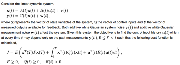
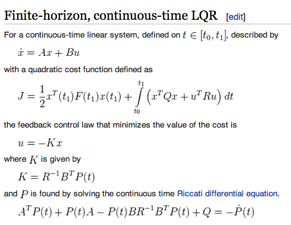
LQG = LQR (control policy) + Kalman filter (LQE state estimation with noisy observables)

Separation principle applies to LQR (control) and Kalman filter (state estimation)


LQR 如下:
NewImage

LQG 如下: 

NewImage


The LQG controller is simply the combination of a Kalman filter i.e. a linear-quadratic estimator (LQE) with a linear-quadratic regulator (LQR).


Markov Decision Policy and LQR 異同

Are they the same things?  It is similar to HMM vs. Kalman filter


LQR

1. continuous states

2. linear space model

3. Gaussian  


Q&A

HMM state is discrete of the PMF -> not significant, 應該是 transition/emission probability matrix PMF 對應 transition/emission Gaussian PDF.

HMM uses Viterbi algorithm to determine the best state like Kalman filter?  No -> Viterbi is the maximum likelihood of state sequence estimator of P(x1, x2, .. xk | y1, y2, .. yk).   Kalman filter is point-like maximum likelihood state estimator P(xk | y1, .. yk).

Determined by the policy function? No -> 完全沒關係


Hidden Markov Model of Filtering, Smoothing – Probabilistic Interpretation

by allenlu2007

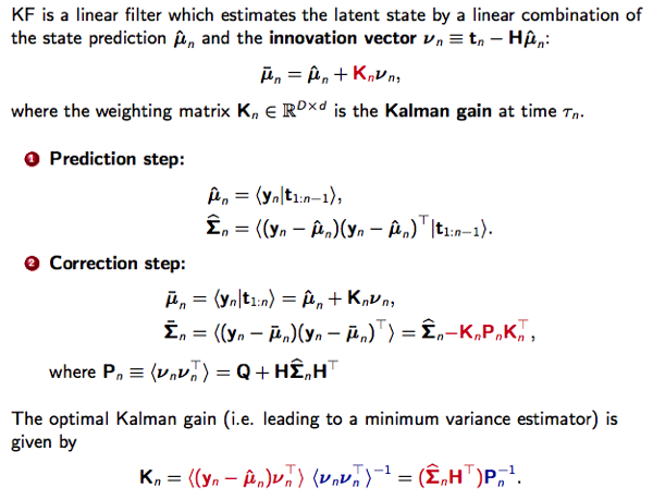
前文 Kalman filter 是從 (linear) state space model 出發:

NewImage


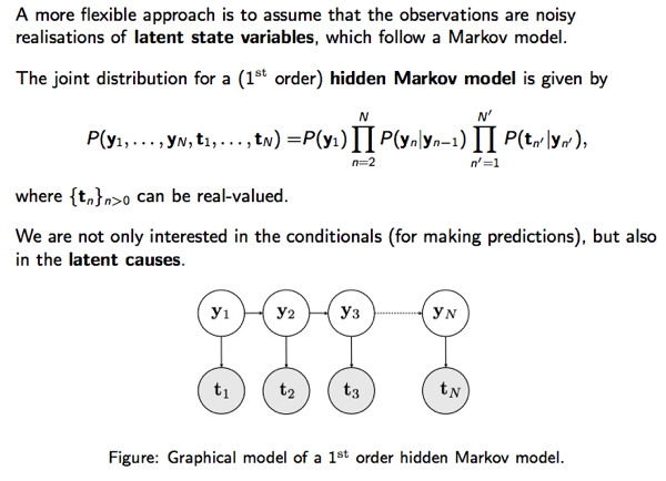
我們可以從 Hidden Markov Model (HMM) 出發,更 general 的 probabilistic model:

Sometimes it is called Bayes filter or recursive Bayesian filter.

Kalman filter 是一個 linear space + Gaussian distribution 的特例。

好處:

1. 更 general

2. 更好的 nonlinear filter or large dimensional filter: Particle filter, Unscented KF, EnKF


The following is reference from xxx

NewImage


上述的 joint PDF 其實是 Bayesian Network (BN) 的直接結果。Joint PDF 等於所有的 conditional PDF product!


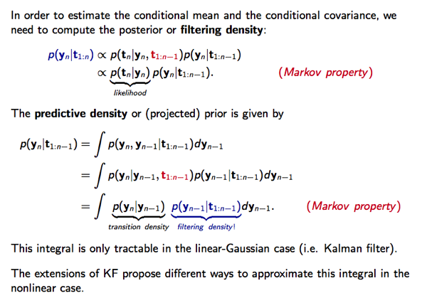
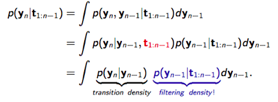
The key to solve the estimation problem is divided into filtering and smoothing!! 

The first equation is directly from Markov property (since t1:n is given, there is only one proportional parameter!)

NewImage

同樣的結論 from another article:

NewImage 

(1) state is X;  output is e

(1a) combine prediction and update into one equation

(2) 多了 smoothing (backward pass).  Smoothing 只有 one step; 不像 filter: prediction+update

(3) summation vs. integration


如何把上述 equation 轉為常見的 Kalman filter and smoother?


Filtering

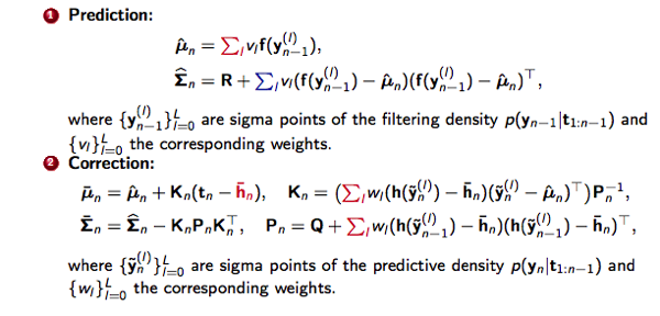
Filtering 分為兩步: prediction and update (or innovation)

Prediction:

(y is state, t is observed data)

NewImage

or ( x is state, z is observed data)

NewImage

or ( x is state, e is observed data)

NewImage


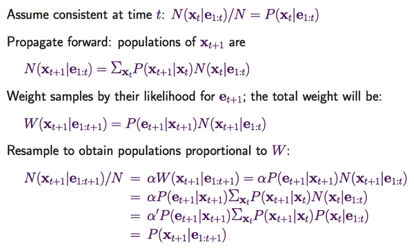
Update (innovation)

NewImage

or more precisely

NewImage

where alpha > 1


Case 1: Linear model : Kalman filter

NewImage

After prediction  …

After update:

NewImage

一個重點是 Kt and Sigma_t 和 observation data 無關,可以 offline compute.  問題是如果 Sigma_x, Sigma_z, 和初始的 Sigma_t 如果不準,所算出的 Kt 自然也不準。可能需要用 EM algorithm 事先 training. 

Or use EnKF to compute the K!


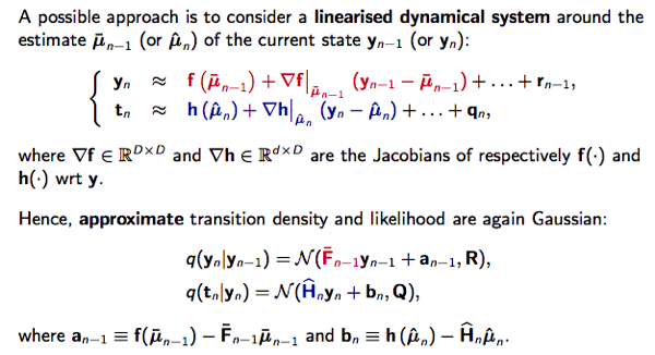
Case 2: Nonlinear model:  Extended Kalman filter (1st order approximation)

如果 nonlinear (therefore non-Gaussian) but well define function with reasonable dimension.

We can use extended Kalman filter.  It is essentially a linear approximation of the nonlinear function.

 NewImage

接下來就和 KF 是一樣的。


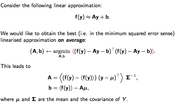
Case 3: Nonlinear model: Unscented Kalman filter (2nd order approximation)

NewImage

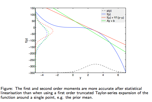
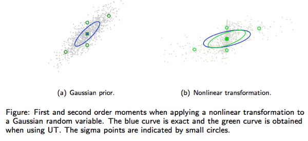
比較 Taylor expansion and statistical linearisation 對 input Gaussian PDF to output 的差異如下圖

NewImage

可以看到 statistical linearisation 所產生的 output PDF 的 1st and 2nd order (mean and variance) 都比 Taylor expansion linearisation 的近似好。這是 unscented KF 的基本概念。

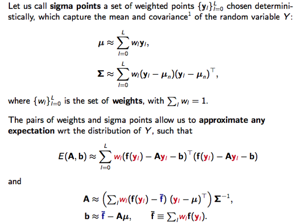
NewImage

NewImage

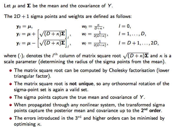
D 是 Gaussian 的 dimension.  1-D 3 points; 2-D 5 points, etc.

NewImage

Sigma point KF 的好處:

* 不需要計算 derivative

* Based on deterministic sampling (非 Monte Carlo)

* Gaussian approximation filter with exact nonlinear models (非 Taylor expansion approximation).  

缺點: 收歛速度比較慢


NewImage


Case 4: particle filter (or sequential Monte Carlo filter)

For nonlinear and non-Gaussian and high dimension case.  There is no well defined nonlinear function.

NewImage


Case 5: Ensemble Kalman filter (EnKF)

A special case of particle filter but everything is Gaussian.  The only problem is high dimensional so it is difficult to compute the covariance matrix.

The EnKF is a monte carlo approximation of the Kalman filter, which avoids evolving the covariance matrix of the state vector x.   K = CH’ (HCH’ + R ) ^ -1

Recall in Kalman filter, Kt and Sigma_t are independent of the observed data (only depends on Q and R)!!  In the EnKF, this is not the case, but it is better because it takes the observed data into account? and avoid the inaccuracy prior assumption of the state covariance?


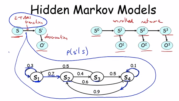
Q: what’s the link of HMM and conventional Markov chain?

   (a) conventional Markov chain (如下), 沒有 show time step, only the state transition and transition probability.

       BTW, the state transition and probability is time invariant.

    (b) conventional Markov chain, the state is directly observable.

    © HMM 的圖如最上。each state circle includes all possible states; and shows the time step transition.


    Answer:  Daphne Kroller 的解釋很清楚 (PGM in coursera).  Conventional Markov chain 定義了 state transition model and transition probability, 而 hidden markov model 代表的是 temporal unroll 的圖。 Markov property and time invariant 是一般 HMM 的 default 假設。  當然 HMM, state 是 unobservable.  

NewImage

NewImage

Kalman Smoother and EM for Stochastic Constant Growth Model

by allenlu2007


以下的例子為 diffusion approximation for a stochastic exponential growth model.  可以用 linear space model 

NewImage

NewImage

 B 是平均 growth rate.  A = C = 1.

NewImage

NewImage

Initial condition t=1

NewImage


再來結合 Markov 的 property (1)

NewImage


and observed output only depends on the corresponding states (2)

NewImage


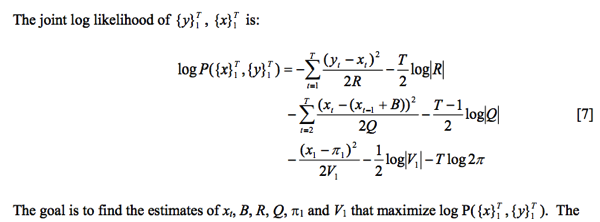
We can get a very simple joint pdf of all Xi and Yi in Kalman filter (or Hidden Markov Model) as!!

NewImage

以下是有趣的部份:

NewImage

Where only Yi are given. 

記住 Xi 是 hidden variables.  因些我們可以(需要)用 EM algorithm 來 optimize


EM Algorithm

由 Shumway and Stoffer (1982) 所建議,基本上有四個步驟。

(0) 計算 initial parameter estimates

NewImage

(1) Kalman smoother: generate an estimate of xt by estimating E(xt | Y1, … YT) given above initial values.

(2) Define  Q function as below.  Update R, Q, B, Pi, V by maximizing the Q function.

NewImage

(3) Check if si function is converged and repeat (1)


以下為分解動作

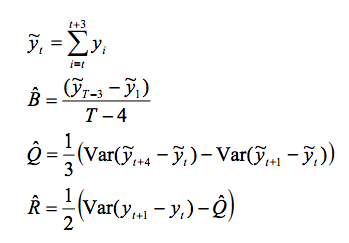
Step 0: Initial Parameter Estimates

By Holmes and Fagan (2002)

NewImage

NewImage


Step 1: Kalman Smoother (Kalman-Rauch Recursion)

NewImage

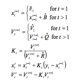
(a)  先用 Kalman filter forward pass to estimate Gaussian pdf of p(xt | y1, .. yt).  

   Gaussian pdf 由 mean and variance 完全決定。Mean (xt = E(xt | y1, .. yt) 和 variance (Vt) 結果如下

NewImage

   Vt 在 prediction phase 時會增加 (by Q), 而在 update phase 時會減小 (by Kt Vt^(t-1))

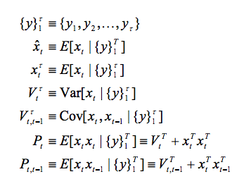
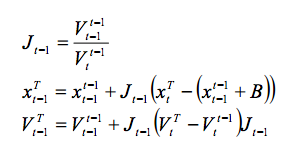
(b) 再用 Rauch backward pass to estimate p(xt| y1, .. yT).  同樣 mean (xt) and variance (Vt) 結果如下

NewImage

   最後一項的右手第二項一般是負的,所以整體的 variance 可以再減少。 

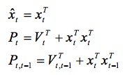
(c) 再一個 backward pass 是計算

NewImage   

NewImage


Step 2: EM Algorithm 

接下來定義 E-step and M-step.  E-step 如下

NewImage

利用在開始所推導的 log P 公式,其實我們不必算出 psi function.

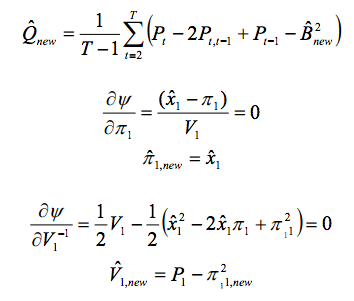
重點在於 taking partial derivative of psi w.r.t. each parameters, set the derivative to zero and solve the maximizing parameter:

NewImage

(好像少了一個 1/T log |R| 的導數? and what is C?)

NewImage

NewImage

Step 3: 檢查收歛性 


Matlab code example

clear all

close all


A = 1

C = 1

B = 0.2

D = 0


t = [0:200];

Q = 0.02;

R = 1;


x0 = 15;


sys = ss(A, B, C, D, -1);


u = ones(length(t), 1);     % external force B*u

v = sqrt(Q)*randn(length(t), 1); %state noise

w = sqrt(R)*randn(length(t), 1); %measurement noise


y = lsim(sys, u+v, t, x0); 

logdata = y + w;


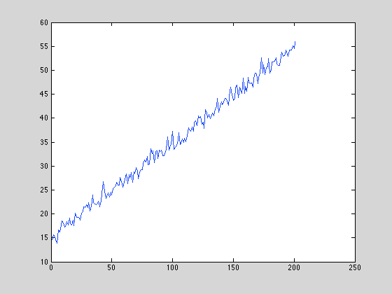
plot(logdata)


[BB, QQ, RR, initx, V1, LL] = PVAKalman(logdata’)


BB = 0.2

RR = 0.9748

QQ = 0.0013

initx = 15.1161


NewImage


EM Algorithm 2:

考慮另一個 model

NewImage

A, B, and C 是已知,但是 Q and R 未知:

NewImage


Kalman Filter, Kalman Smoother, and Expectation Maximization

by allenlu2007


前文提到 Kalman filter 的好處 (i) 探索 data 的內在結構 (state equation and noise covariance matrix), 以及 (ii) 發展出 recursive equation 來 estimate 內在的結構 (state or sometimes noise).

實際上遇到的困難是 (a) 這樣的 state equation 是否存在? (b) 如果存在如何找到正確的 model 參數? and (c) 如果 model or 參數不準確,Kalman filter estimate 的結果是否 robust?

(a) State equation 是否存在

有兩種解釋: (i) state equation bases on physics  如力學、電子學、etc. (ii) dynamic system 的線性近似。

(b) 如何找到 model 的參數

(i) 由 equation 推導出. (ii) 是由 training 出來的。如果是 (ii) 一般不會差太多。

(c) 如果 model or 參數不準確,Kalman filter estimate 的結果是否 robust?

Again, 可能要用 training 方式來找 Kalman filter 的 Q, R, A, C.  避免 Kalman filter output 和現實差太多。


Kalman filter Training (parameter estimation) 的方式可以用 EM algorithm 或其他 system identification algorithm (ARMA, .. etc.)

Kalman filter is typically used for on-line state estimation and a minimum-variance smoother may be employed for off-line or batch state estimation. However, these minimum-variance solutions require estimates of the state-space model parameters. EM algorithms can be used for solving joint state and parameter estimation problems.

1. 似乎是 Kalman smoother 才可以。Kalman filter 不能?  是因為必須 batch mode?


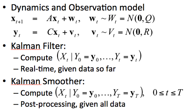
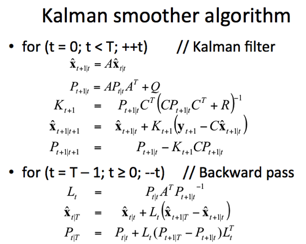
Step 0: Kalman filter and Kalman smoother 的差異如下:

(a) Kalman filter 主要是”當下”的最佳 estimation.  依照 Markov state 的定義,只要有前一 state 的 pdf/information (mean and covariance matrix; mean 是 x_hat; covariance matrix 是 P), 就可以 ignore 更早的 information.  

(b) Kalman smoother 則是用未來的 observed data 來回推最佳的 estimation.  By the same token, 似乎只要”下一個” sample 就足夠。實則不然,因為需要的是下一 state 的 pdf/information, 並非只是 observed data.  下一 state 的 pdf/information 可以被 estimate 更精確如果知道下下 sample (because they are correlated), 依此類推。當然也可以只看下一個 (或下幾個) sample 來做 Kalman smoother, 稱為 fixed-length or fixed-interval smoothing.  只是所得到的 variance reduction 不是最佳。實務上很少在 real time application 用 Kalman smoother, 主要是 complexity 以及額外的 latency for smoothing.

NewImage

Step 1: Kalman smoother State Estimation:

因此完整的 Kalman smoother 需要所有的 data 來做 post-processing (Viterbi 例外?)


NewImage

對 Kalman filter 來說,xt 是一個 Gaussian random variable.  Mean 是 x_hat; covariance matrix 是 P.  P 在 prediction 時增加 (if Q>0),在 update 時減小。

Kalman smoother 多了 backward pass 可以給更好的 estimation, covariance matrix 應該要減小.  此時並非 real time.  理論上 Pt|T < Pt|t (how to prove?)

Find an example to show the difference of Kalman filter and Kalman smoother!


Step 3: EM algorithm of State Estimation

綜上所述 Kalman smoother 的 state estimation (mean and covariance) 優於 Kalman filter.  Trade-off 是 complexity and latency.  對於 real-time applications 如 tracking, navigation, etc., Kalman filter 比較適合。但若是一些非 real-time 的影像或聲音處理,Kalman smoother 可以多得到一些 performance.  

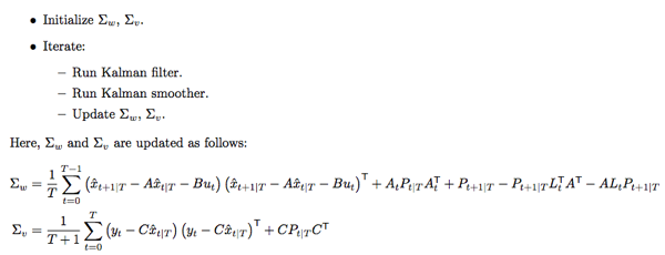
Kalman smoother 其實還有一個重要的應用,就是配合 EM algorithm, 用來 estimate A, C, Q, R (當然同時 estimate state 的 mean and covariance)! Magic!

因為在實務上,Q and R 大多非 prior information (如何事先知道 state noise and measurement noise 的大小?) 因此可以靠 training (with or without prior state information).  更進一步,有時 A and C 也是 unknown, 也需要由 training 而來。

結合 EM algorithm 和 Kalman smoother 可以做為 training (without prior state information!!) 而得到 A, C, Q, R 的 estimation.  再 performance real-time Kalman filter.   

EM 的 E-step 就是 Kalman smoother.  M-step 就是 update A, C, Q, R based on ML estimation.  EM algorithm 需要解決兩個問題: (i) 如何決定 A, C, Q, R 的 initial guess.  (ii) 如何避免 local minimum.

NewImage


Example: 


Kalman filter, LQR, LQG, and Separation Principle

by allenlu2007


From Andrew Ng lecture


Kalman filter is to estimate state

LQR is to obtain the optimal control policy

It turns out in Kalman filter case; estimate state is optimal for the optimal control policy,

namely LQG  – linear quadratic gaussian

This is also called the separation principle – estimation and control can separate independently.


LQR can ignore state noise

LQG can additionally ignore the observation noise

separation principle!!


From Princeton Stigel’s note


From MIT underactuated Robotics!! Excellent lecture by Russ Tedrake 

Very good in control.  Use a simple pendulum as a base example. 

Explore to different control algorithms for nonlinear dynamic 

–> nonlinear dynamics Chaos by Steve Strogatz

Simple pendulum

Lagrange: generalized force to model friction (damping)

Impact 

— limit cycle


Optimal control 

— analytical OC

— numerical OC based on DP


Numerical OC based on policy search


More EM Examples

by allenlu2007

Based on Andrew Ng’s lecture, there are more applications for EM algorithm.


1.  GMM: done in the previous article

2.  Naive Bayesian Mixture:  Two types:   multivariate binomial mixture;  multinomial mixture: commonly used in machine learning.

3.  Factor analysis: to reduce the dimension of observed data  (http://newgenerationresearcher.blogspot.tw/2009/02/factor-analysis.html)


以及其他的包含

* Kalman filter 的 A, C, Q, R estimation.

* Hidden markov model (HMM) 的 estimation? Baum Welch algorithm  (和以上應該是同一件事?)

* Possion random process: wavefront sensing


Machine Learning Lecture

by allenlu2007

這幾天把 Stanford CS229 Andrew Ng 的 machine learning lecture 看了一半,有幾點感想。

1. Ng 的理論背景扎實,lecture handout 都很清楚。每個証明的策略和細節他都一一走過,非常不容易。至少我做不到。

2. 不過有些部份以乎還不夠深入。例如牛頓法在最小值為什麼收歛比 gradient descent 快。object function with regulation 的 trade-off. Boyd 的 convex optimisation lecture 說的更深入。兩者有互補作用。

2a. supervise learning 的 ML 的 parameter estimation 是 maximize joint likelihood function 而非 conditional likelihood functions.  這點很重要!!  結論是 ML parameter estimation 就是要 maximise 所有 observed data 的 probability.  In supervise training 的 training phase,  both input and output are observed, 所以當然是 maximise joint likelihood.  但在一般的 parameter estimation, internal state or unsupervised learning case, 只有 output 是 observed, 所以 maximise conditional likelihood.

3. Ng 解釋很好的部份有: logistic regression, support vector machine,  machine learning debugging (high bias or high variance, algorithm convergence problem or objective function problem, etc.)  特別他解釋 expectation maximisation 部份讓我之前對於整個 logic 更清楚的了解。之後再整理這部份。

4. 交互比較 Ng and Boyd 的 lecture and note 應該可以收獲更多。